Can we use Base R to find the 95% of the area under a curve?

Question

Using Base R, I was wondering if I could determine the 95% area under the curve denoted as posterior below?

More specifically, I want to move from the mode (the green dashed line) toward the tails and then stop when I have covered 95% of the curve area. Desired are the x-axis values that are the limits of this 95% area as shown in the picture below?

     prior = function(x) dbeta(x, 15.566, 7.051) 
likelihood = function(x) dbinom(55, 100, x)
 posterior = function(x) prior(x)*likelihood(x)

mode = optimize(posterior, interval = c(0, 1), maximum = TRUE, tol = 1e-12)[[1]]

curve(posterior, n = 1e4)

P.S In other words, it is highly desirable if such an Interval be the shortest 95% interval possible.

Monoplane

Answer 1

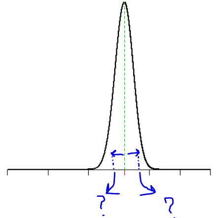
Symmetric distribution

Even though OP's example was not exactly symmetric, it is close enough - and useful to start there since the solution is much simpler.

You can use a combination of integrate and optimize. I wrote this as a custom function, but note that if you use this in other situations you may have to rethink the bounds for searching the quantile.

# For a distribution with a single peak, find the symmetric!
# interval that contains probs probability. Search over 'range'.
f_quan <- function(fun, probs, range=c(0,1)){

  mode <- optimize(fun, interval = range, maximum = TRUE, tol = 1e-12)[[1]]

  total_area <- integrate(fun, range[1], range[2])[[1]]

  O <- function(d){
    parea <- integrate(fun, mode-d, mode+d)[[1]] / total_area
    (probs - parea)^2
  }
  # Bounds for searching may need some adjustment depending on the problem!
  o <- optimize(O, c(0,range[2]/2 - 1E-02))[[1]]

return(c(mode-o, mode+o))
}

Use it like this,

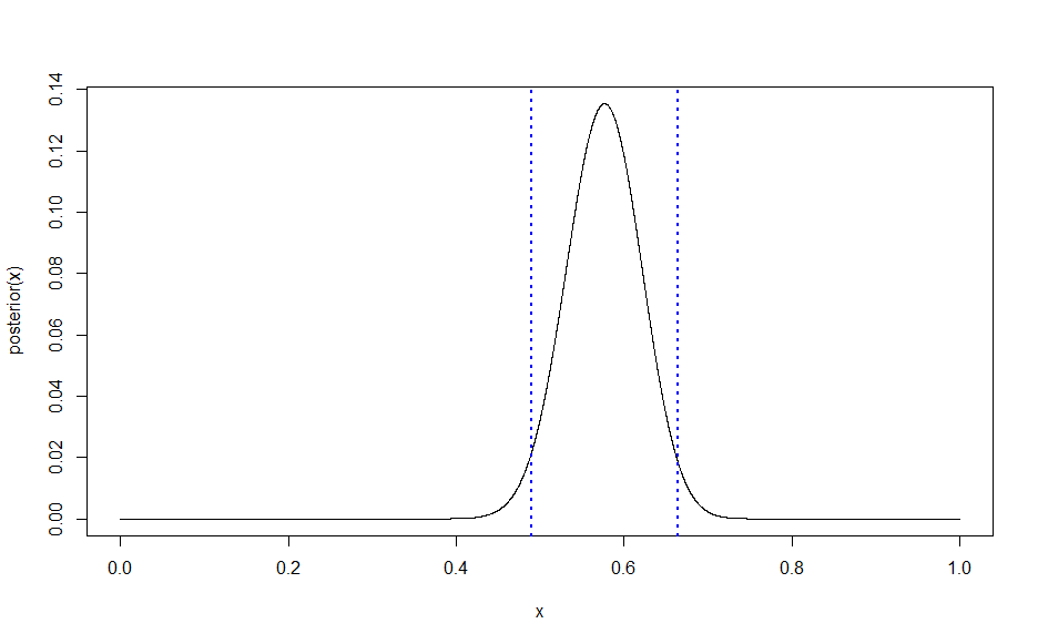
f <- f_quan(posterior, 0.95)
curve(posterior, n = 1e4)
abline(v=f, col="blue", lwd=2, lty=3)

gives

Asymmetric distribution

In the case of an asymmetric distribution, we have to search two points that meet the criterium that P(a < x < b) = Prob, where Prob is some desired probability. Since there are infinitely many intervals (a,b) that meet this, OP suggested finding the shortest one.

Important in the solution is the definition of a domain, the region where we want to search (we cannot use -Inf, Inf, so the user has to set this to reasonable values).

# consider interval (a,b) on the x-axis
# integrate our function, normalize to total area, to 
# get the total probability in the interval
prob_ab <- function(fun, a, b, domain){
  totarea <- integrate(fun, domain[1], domain[2])[[1]]
  integrate(fun, a, b)[[1]] / totarea
}

# now given a and the probability, invert to find b
invert_prob_ab <- function(fun, a, prob, domain){

  O <- function(b, fun, a, prob){
    (prob_ab(fun, a, b, domain=domain) - prob)^2
  }

  b <- optimize(O, c(a, domain[2]), a = a, fun=fun, prob=prob)$minimum

return(b)
}

# now find the shortest interval by varying a
# Simplification: don't search past the mode, otherwise getting close
# to the right-hand side of domain will give serious trouble!
prob_int_shortest <- function(fun, prob, domain){

  mode <- optimize(fun, interval = domain, maximum = TRUE, tol = 1e-12)[[1]]

  # objective function to be minimized: the width of the interval
  O <- function(a, fun, prob, domain){
    b <- invert_prob_ab(fun, a, prob, domain)

    b - a
  }

  # shortest interval that meets criterium
  abest <- optimize(O, c(0,mode), fun=fun, prob=prob, domain=domain)$minimum

  # now return the interval
  b <- invert_prob_ab(fun, abest, prob, domain)

return(c(abest,b))
}

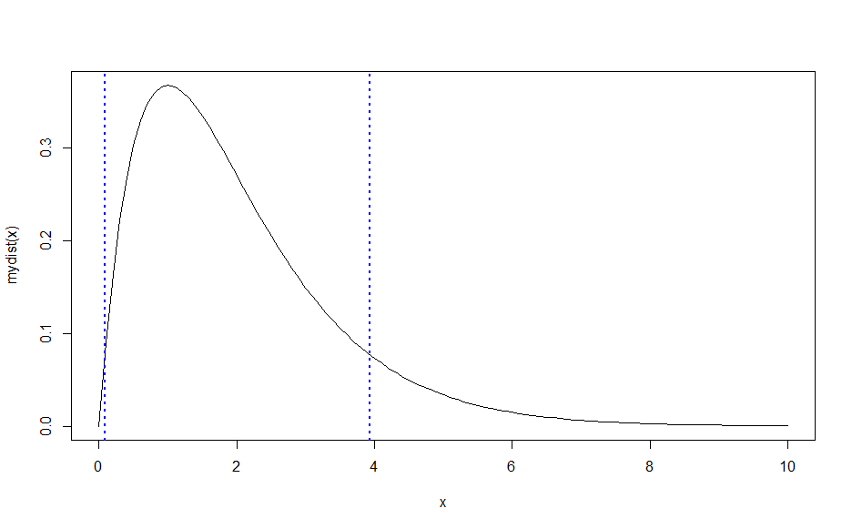
Now use the above code like this. I use a very asymmetric function (just assume mydist is actually some complicated pdf, not the dgamma).

mydist <- function(x)dgamma(x, shape=2)
curve(mydist(x), from=0,  to=10)
abline(v=prob_int_shortest(mydist, 0.9, c(0,10)), lty=3, col="blue", lwd=2)

In this example I set domain to (0,10), since clearly the interval must be in there somewhere. Note that using a very large value like (0, 1E05) does not work, because integrate has trouble with long sequences of near-zeroes. Again, for your situation, you will have to adjust the domain (unless someone has a better idea!).

Powell

The bounds are the issue: if you search across the entire domain (0-1 in your case), we get problems since the function is not defined at 0 or 1 (but it is nearby). In the function d is the distance from the mode, this is varied so as to find the d where integral of (mode-d) to (mode+d) is equal to the probability requested (0.95 in your case). Hence this only works for symmetric functions, otherwise you'd have to optimize two parameters. – Powell

I think if it is asymmetric, there is not going to be a single solution to this problem! You can find many intervals for a pdf that integrates to some probability. Or, are you actually looking for the 2.5% and 97.% quantiles (which would integrate to 95% in between those)? If so, that can be done. – Powell

That can be done - but mind you that is quite different from the original question you asked! I hesitate to edit my post since that is useful in its own right. I might add another answer. – Powell

Remko, I agree with OP your edited answer will be highly useful, and even more upvote getter. – Suu

Answer 2

Here is a solution making use of the Trapezoidal rule. You will note that the solution provided by @Remko is far superior, however this solution hopefully adds some pedagogical value as it illuminates how complicated problems can be reduced to simple geometry, arithmetic, and basic programming constructs such as for loops.

findXVals <- function(lim, p) {
    ## (1/p) is the precision

    ## area of a trapezoid
    trapez <- function(h1, h2, w) {(h1 + h2) * w / 2}

    yVals <- posterior((1:(p - 1))/p)
    m <- which.max(yVals)
    nZ <- which(yVals > 1/p)

    b <- m + 1
    e <- m - 1
    a <- f <- m

    area <- 0
    myRng <- 1:(length(nZ)-1)
    totArea <- sum(trapez(yVals[nZ[myRng]], yVals[nZ[myRng+1]], 1/p))
    targetArea <- totArea * lim

    while (area < targetArea) {
        area <- area + trapez(yVals[a], yVals[b], 1/p) + trapez(yVals[e], yVals[f], 1/p)
        a <- b
        b <- b + 1
        f <- e
        e <- e - 1
    }

    c((a - 1)/p, (f + 1)/p)
}

findXVals(.95, 10^5)
[1] 0.66375 0.48975

Blockhouse