How to find Local maxima in Kernel Density Estimation?

Question

I'm trying to make a filter (to remove outlier and noise) using kernel density estimators(KDE). I applied KDE in my 3D (d=3) data points and that gives me the probability density function (PDF) f(x). Now as we know local maxima of density estimation f(x) defined the centers of the clusters of data points. So my idea is to define the appropriate f(x) which will determine those clusters.

My question is how and what method will be better suited for this purpose of finding local maxima in f(x). If anyone can provide me some example code/ idea I will really appreciate it.

Here is the code to find the KDE which give f(x) in 3D data.

import numpy as np
from scipy import stats

data = np.array([[1, 4, 3], [2, .6, 1.2], [2, 1, 1.2],
         [2, 0.5, 1.4], [5, .5, 0], [0, 0, 0],
         [1, 4, 3], [5, .5, 0], [2, .5, 1.2]])
data = data.T 
kde = stats.gaussian_kde(data)
minima = data.T.min(axis=0)
maxima = data.T.max(axis=0)
space = [np.linspace(mini,maxi,20) for mini, maxi in zip(minima,maxima)]
grid = np.meshgrid(*space)
coords = np.vstack(map(np.ravel, grid))
#Evaluate the KD estimated pdf at each coordinate
density = kde(coords)

Octahedron

Answer 1

Here is a short function that demonstrates how you could estimate the maxima. Note: the higher the number of no_samples the more accurate the maxima.

from scipy.stats import gaussian_kde
import numpy as np

 def estimate_maxima(data):
    kde = gaussian_kde(data)
    no_samples = 10
    samples = np.linspace(min(data), max(data), no_samples)
    probs = kde.evaluate(samples)
    maxima_index = probs.argmax()
    maxima = samples[maxima_index]
    
    return maxima

Abbotsen

The samples assumes data is spread between 0-10, it should be: samples = np.linspace(min(data), max(data), no_samples) – Fidelis

Answer 2

You will want to use an algorithm called Mean Shift. Its a clustering algorithm that works by finding the modes (aka maxima of f(x)) of the KDE. Note that the bandwidth set for your KDE will impact the number of modes and their locations. Since you are using python, there is an implementation in scikit-learn.

Cthrine

thanks for the idea. I followed your advice and applied meanshift to my density value. but I'm not sure how to get local maxima. its giving me 6 clusters :( . here is the Source Code, Am I doing it right? – Octahedron

The cluster_centers should contain the maxima, as a "center" doesn't make much sense since the cluster shape can be very irregular. – Cthrine

Extremely slow on moderately big data (1e4) – Cenotaph

Yes, Python is quite slow - as is the default scikit implementation. It has a simple binning option that will help, and there are other approaches to faster mean shift. – Cthrine

Answer 3

You could use scipy.optimize.

Example on 1D-data:

import numpy as np
from scipy import optimize
from scipy import stats


# Generate some random data
shape, loc, scale = .5, 3, 10
n = 1000
data = np.sort(stats.lognorm.rvs(shape, loc, scale, size=n))

kernel = stats.gaussian_kde(data)
# Minimize the negative instead of maximizing
# Depending on the shape of your data, you might want to set some bounds
opt = optimize.minimize_scalar(lambda x: -kernel(x))
opt

     fun: array([-0.08363781])
    nfev: 21
     nit: 14
 success: True
       x: array([10.77361776])

The actual mode of this distribution is at

mode = scale/np.exp(shape**2) + loc
mode
10.788007830714049

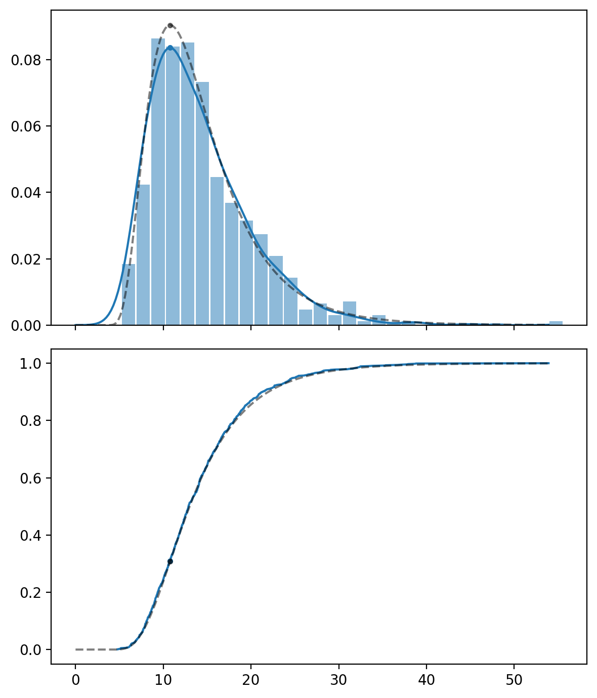
Plotting the results:

import matplotlib.pyplot as plt

data_es = np.linspace(0, data.max(), 201)  # x-axis points
ecdf = (np.arange(n) + 1)/n  # empirical CDF

fig, axes = plt.subplots(2, 1, sharex=True, dpi=300, figsize=(6,7))
axes[0].hist(x, bins=30, density=True, alpha=.5, rwidth=.9)  # histogram
axes[0].plot(data_es, kernel.pdf(data_es), 'C0')  # estimated PDF
axes[0].plot(data_es, stats.lognorm.pdf(data_es, shape, loc, scale), 'k--', alpha=.5)  # true PDF
axes[0].plot(opt.x, kernel.pdf(opt.x), 'C0.')  # estimated mode
axes[0].plot(mode, stats.lognorm.pdf(mode, shape, loc, scale), 'k.', alpha=.5)  # true mode

axes[1].plot(np.sort(data), ecdf)  # estimated CDF
axes[1].plot(opt.x, np.interp(opt.x, np.sort(data), ecdf), 'C0.')  #estimated mode
axes[1].plot(data_es, stats.lognorm.cdf(data_es, shape, loc, scale), 'k--', alpha=.5)  # true CDF
axes[1].plot(mode, stats.lognorm.cdf(mode, shape, loc, scale), 'k.', alpha=.5)  # true mode

fig.tight_layout()

As you can see, the estimated mode fits pretty well. I assume it can be expanded to multi-variate data with other methods from scipy.optimize.

Flattish