Measuring the similarity between two irregular plots

Question

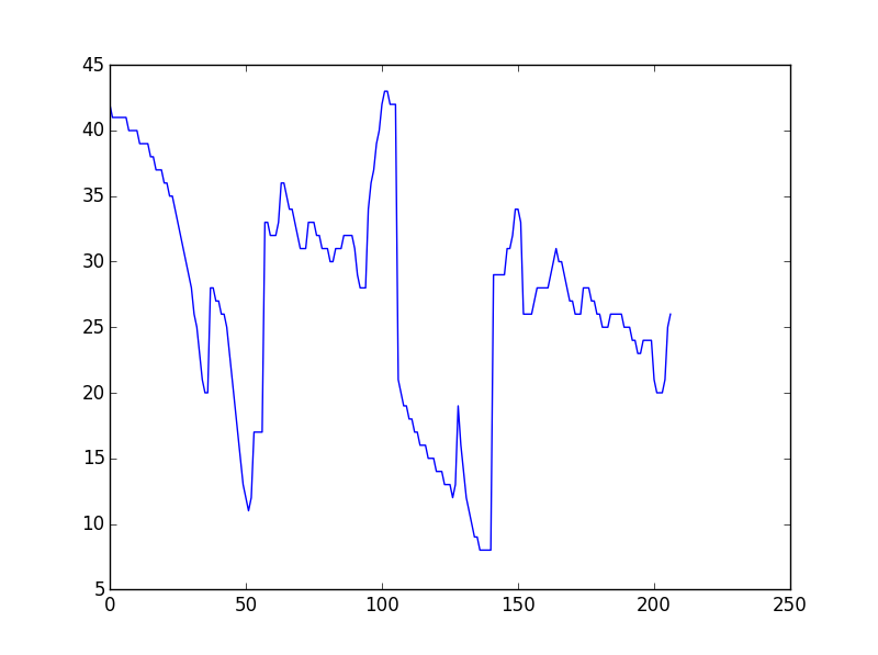
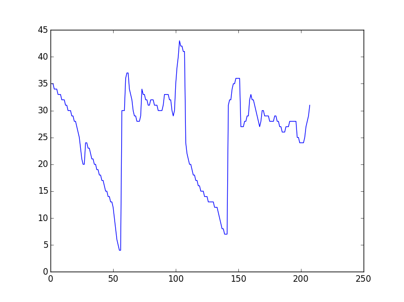
I have two irregular lines as a list of [x,y] coordinates, which has peaks and troughs. The length of the list might vary slightly(unequal). I want to measure their similarity such that to check occurence of the peaks and troughs (of similar depth or height) are coming at proper interval and give a similarity measure. I want to do this in Python. Is there any inbuilt function to do this?

Sarabia

What's similar; are you looking for exact match? Do the lists of points have to be in order, or can you reorder them? – Lynsey

Not exact but pattern match measurement. It has to be in order – Sarabia

Are your data points equally spaced on the x-axis? – Maulstick

I have posted two images in question...can u see some sort of pattern in it. How can that pattern similarity be measured? – Sarabia

Answer 1

I don't know of any builtin functions in Python to do this.

I can give you a list of possible functions in the Python ecosystem you can use. This is in no way a complete list of functions, and there are probably quite a few methods out there that I am not aware of.

If the data is ordered, but you don't know which data point is the first and which data point is last:

1. Use the directed Hausdorff distance

If the data is ordered, and you know the first and last points are correct:

1. Discrete Fréchet distance ^*
2. Dynamic Time Warping (DTW) ^*
3. Partial Curve Mapping (PCM) ^**
4. A Curve-Length distance metric (uses arc length distance from beginning to end) ^**
5. Area between two curves ^**

^* Generally mathematical method used in a variety of machine learning tasks

^** Methods I've used to identify unique material hysteresis responses

First let's assume we have two of the exact same random X Y data. Note that all of these methods will return a zero. You can install the similaritymeasures from pip if you do not have it.

import numpy as np
from scipy.spatial.distance import directed_hausdorff
import similaritymeasures
import matplotlib.pyplot as plt

# Generate random experimental data
np.random.seed(121)
x = np.random.random(100)
y = np.random.random(100)
P = np.array([x, y]).T

# Generate an exact copy of P, Q, which we will use to compare
Q = P.copy()

dh, ind1, ind2 = directed_hausdorff(P, Q)
df = similaritymeasures.frechet_dist(P, Q)
dtw, d = similaritymeasures.dtw(P, Q)
pcm = similaritymeasures.pcm(P, Q)
area = similaritymeasures.area_between_two_curves(P, Q)
cl = similaritymeasures.curve_length_measure(P, Q)

# all methods will return 0.0 when P and Q are the same
print(dh, df, dtw, pcm, cl, area)

The printed output is 0.0, 0.0, 0.0, 0.0, 0.0, 0.0 This is because the curves P and Q are exactly the same!

Now let's assume P and Q are different.

# Generate random experimental data
np.random.seed(121)
x = np.random.random(100)
y = np.random.random(100)
P = np.array([x, y]).T

# Generate random Q
x = np.random.random(100)
y = np.random.random(100)
Q = np.array([x, y]).T

dh, ind1, ind2 = directed_hausdorff(P, Q)
df = similaritymeasures.frechet_dist(P, Q)
dtw, d = similaritymeasures.dtw(P, Q)
pcm = similaritymeasures.pcm(P, Q)
area = similaritymeasures.area_between_two_curves(P, Q)
cl = similaritymeasures.curve_length_measure(P, Q)

# all methods will return 0.0 when P and Q are the same
print(dh, df, dtw, pcm, cl, area)

The printed output is 0.107, 0.743, 37.69, 21.5, 6.86, 11.8 which quantify how different P is from Q according to each method.

You now have many methods to compare the two curves. I would start with DTW, since this has been used in many time series applications which look like the data you have uploaded.

We can visualize what P and Q look like with the following code.

plt.figure()
plt.plot(P[:, 0], P[:, 1])
plt.plot(Q[:, 0], Q[:, 1])
plt.show()

Gillie

Answer 2

Since your arrays are not the same size ( and I am assuming you are taking the same real time) , you need to interpolate them to compare across related set of points. The following code does that, and calculates correlation measures:

#!/usr/bin/python
import numpy as np
from scipy.interpolate import interp1d
import matplotlib.pyplot as plt
import scipy.spatial.distance as ssd 
import scipy.stats as ss

x = np.linspace(0, 10, num=11)
x2 = np.linspace(1, 11, num=13)

y = 2*np.cos( x) + 4 + np.random.random(len(x))
y2 = 2* np.cos(x2) + 5 + np.random.random(len(x2))

# Interpolating now, using linear, but you can do better based on your data
f = interp1d(x, y)
f2 = interp1d(x2,y2)

points = 15

xnew = np.linspace ( min(x), max(x), num = points) 
xnew2 = np.linspace ( min(x2), max(x2), num = points) 

ynew = f(xnew) 
ynew2 = f2(xnew2) 
plt.plot(x,y, 'r', x2, y2, 'g', xnew, ynew, 'r--', xnew2, ynew2, 'g--')
plt.show()

# Now compute correlations
print ssd.correlation(ynew, ynew2) # Computes a distance measure based on correlation between the two vectors
print np.correlate(ynew, ynew2, mode='valid') # Does a cross-correlation of same sized arrays and gives back correlation
print np.corrcoef(ynew, ynew2) # Gives back the correlation matrix for the two arrays

print ss.spearmanr(ynew, ynew2) # Gives the spearman correlation for the two arrays

Output:

0.499028272458

[ 363.48984942]

[[ 1.          0.50097173]
 [ 0.50097173  1.        ]]

SpearmanrResult(correlation=0.45357142857142857, pvalue=0.089485900143027278)

Remember that the correlations here are parametric and pearson type and assume monotonicity for calculating correlations. If this is not the case, and you think that your arrays are just changing sign together, you can use Spearman's correlation as in the last example.

Maulstick

Answer 3

I'm not aware of an inbuild function, but sounds like you can modify Levenshtein's distance. The following code is adopted from the code at wikibooks.

def point_distance(p1, p2):
    # Define distance, if they are the same, then the distance should be 0


def levenshtein_point(l1, l2):
    if len(l1) < len(l2):
        return levenshtein(l2, l1)

    # len(l1) >= len(l2)
    if len(l2) == 0:
        return len(l1)

    previous_row = range(len(l2) + 1)
    for i, p1 in enumerate(l1):
        current_row = [i + 1]
        for j, p2 in enumerate(l2):
            print('{},{}'.format(p1, p2))
            insertions = previous_row[j + 1] + 1 # j+1 instead of j since previous_row and current_row are one character longer
            deletions = current_row[j] + 1       # than l2
            substitutions = previous_row[j] + point_distance(p1, p2)
            current_row.append(min(insertions, deletions, substitutions))
        previous_row = current_row

    return previous_row[-1]

Lynsey