Differentiable round function in Tensorflow?

Question

So the output of my network is a list of propabilities, which I then round using tf.round() to be either 0 or 1, this is crucial for this project. I then found out that tf.round isn't differentiable so I'm kinda lost there.. :/

Hulky

Answer 1

Rounding is a fundamentally nondifferentiable function, so you're out of luck there. The normal procedure for this kind of situation is to find a way to either use the probabilities, say by using them to calculate an expected value, or by taking the maximum probability that is output and choose that one as the network's prediction. If you aren't using the output for calculating your loss function though, you can go ahead and just apply it to the result and it doesn't matter if it's differentiable. Now, if you want an informative loss function for the purpose of training the network, maybe you should consider whether keeping the output in the format of probabilities might actually be to your advantage (it will likely make your training process smoother)- that way you can just convert the probabilities to actual estimates outside of the network, after training.

Brockman

My output has to be a value of 1 or 0. But because most of the outputs in the training data are 0 the network just learns to output mostly very low valueds from 0 - 0.0001 and I'm really kinda lost here. So I thought forcing it to output either a 1 or 0 would help.. I thought about just putting a 1 instead of where the derivative of the round function is supposed to be, but then again I use Tensorflow I can't decide the derivatives – Hulky

In that case, the solution should be to oversample the data so that 50% is 1 and 50% is 0. Than it wouldn't matter, because you would eliminate the problem entirely by giving the same number of 0 and 1 on the output – Vaunting

Answer 2

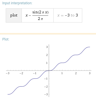
Something along the lines of x - sin(2pi x)/(2pi)?

I'm sure there's a way to squish the slope to be a bit steeper.

Actinouranium

This is an underrated answer. Sincerely, -someone who needed all reals; not just [0,1] – Hardset

I agree this answer is very useful. When something is not possible, use approximation. – Hosea

This idea is amazing, but in my code I tweaked it for slightly better differentiation properties: x/2 - sin(2pi x)/(4pi). It has the same basic shape, but the derivative at 0.5n = 1, so it should converge nicer. For reference, I did this by integrating (1 - cos(2pi))/2, which is a sine wave oscillating between 0 and 1 – Pancreas

@Pancreas that's no longer an answer to the question since it's not "rounding" but "rounding and halving" -- though the scaling of the values and the derivatives would be taken care of at some point by any practical application so i don't think it matters either way – Actinouranium

Answer 3

You can use the fact that tf.maximum() and tf.minimum() are differentiable, and the inputs are probabilities from 0 to 1

# round numbers less than 0.5 to zero;
# by making them negative and taking the maximum with 0
differentiable_round = tf.maximum(x-0.499,0)
# scale the remaining numbers (0 to 0.5) to greater than 1
# the other half (zeros) is not affected by multiplication
differentiable_round = differentiable_round * 10000
# take the minimum with 1
differentiable_round = tf.minimum(differentiable_round, 1)

Example:

[0.1,       0.5,     0.7]
[-0.0989, 0.001, 0.20099] # x - 0.499
[0,       0.001, 0.20099] # max(x-0.499, 0)
[0,          10,  2009.9] # max(x-0.499, 0) * 10000
[0,         1.0,     1.0] # min(max(x-0.499, 0) * 10000, 1)

Locarno

Cool answer! Though has anyone tried using this to train models? Sounds very complicated and I hope models can converge. – Hosea

Now that I tried implementing it, I am not sure it will work. The issue about step function is not that we cannot represent it in tensorflow, but rather it is nondifferentiable. Finding a way to represent it using differentiable operator would still give you a nondifferentiable function. – Hosea

Same here, I tried implementing this but the model's loss was constant. Seems the model can't converge with this kind of function. – Myrmeco

Answer 4

This works for me:

x_rounded_NOT_differentiable = tf.round(x)
x_rounded_differentiable = x - tf.stop_gradient(x - x_rounded_NOT_differentiable)

Stutz

Answer 5

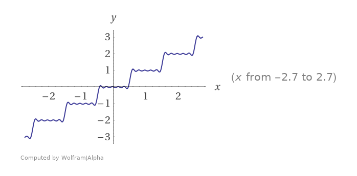
Building on a previous answer, a way to get an arbitrarily good approximation is to approximate round() using a finite Fourier approximation and use as many terms as you need. Fundamentally, you can think of round(x) as adding a reverse (i. e. descending) sawtooth wave to x. So, using the Fourier expansion of the sawtooth wave we get

With N = 5, we get a pretty nice approximation:

Outfox

It's certainly differentiable but the gradient is very non-monotonic so I'm not sure it's useful for most purposes. – Actinouranium

Answer 6

Kind of an old question, but I just solved this problem for TensorFlow 2.0. I am using the following round function on in my audio auto-encoder project. I basically want to create a discrete representation of sound which is compressed in time. I use the round function to clamp the output of the encoder to integer values. It has been working well for me so far.

@tf.custom_gradient
def round_with_gradients(x):
    def grad(dy):
        return dy
    return tf.round(x), grad

Rafaelita

Answer 7

In tensorflow 2.10, there is a function called soft_round which achieves exactly this.

Fortunately, for those who are using lower versions, the source code is really simple, so I just copy-pasted those lines, and it works like a charm:

def soft_round(x, alpha, eps=1e-3):
    """Differentiable approximation to `round`.

    Larger alphas correspond to closer approximations of the round function.
    If alpha is close to zero, this function reduces to the identity.

    This is described in Sec. 4.1. in the paper
    > "Universally Quantized Neural Compression"<br />
    > Eirikur Agustsson & Lucas Theis<br />
    > https://arxiv.org/abs/2006.09952

    Args:
    x: `tf.Tensor`. Inputs to the rounding function.
    alpha: Float or `tf.Tensor`. Controls smoothness of the approximation.
    eps: Float. Threshold below which `soft_round` will return identity.

    Returns:
    `tf.Tensor`
    """
    # This guards the gradient of tf.where below against NaNs, while maintaining
    # correctness, as for alpha < eps the result is ignored.
    alpha_bounded = tf.maximum(alpha, eps)


    m = tf.floor(x) + .5
    r = x - m
    z = tf.tanh(alpha_bounded / 2.) * 2.
    y = m + tf.tanh(alpha_bounded * r) / z


    # For very low alphas, soft_round behaves like identity
    return tf.where(alpha < eps, x, y, name="soft_round")

alpha sets how soft the function is. Greater values leads to better approximations of round function, but then it becomes harder to fit since gradients vanish:

x = tf.convert_to_tensor(np.arange(-2,2,.1).astype(np.float32))

for alpha in [ 3., 7., 15.]:

    y = soft_round(x, alpha)
    plt.plot(x.numpy(), y.numpy(), label=f'alpha={alpha}')

plt.legend()
plt.title('Soft round function for different alphas')
plt.grid()

In my case, I tried different values for alpha, and 3. looks like a good choice.

Ejective

Answer 8

In range 0 1, translating and scaling a sigmoid can be a solution:

  slope = 1000
  center = 0.5
  e = tf.exp(slope*(x-center))
  round_diff = e/(e+1)

Woald

Answer 9

You can simply approximate rounding (thus differentiable) using this function

def diff_round(x):
    return torch.round(x) + (x - torch.round(x))**3

Replace torch.round with diff_round

Madura

Answer 10

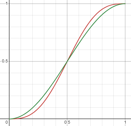
To expand upon the answer with sin(2πx): if you want the function to be slightly less flat near the integers and you don't need it for inputs beyond [0,1], you can forego adding x and just use 0.5*cos(πx-π) + 0.5. The red curve is x - sin(2πx)/(2πx), the green curve is that cosine.

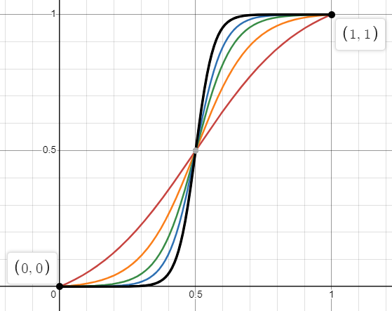
Alternatively, you can use a scaled and shifted sigmoid such that it intersects (0,0) and (1,1). The advantage is that unlike a sine or cosine, you can control how steep the curve flows between those fixed points (you can't with sine and cosine because their steepness also changes where they have their roots).

A basic sigmoid is 1/(1 + exp(-x)). Shifting to have it intersect y = 0.5 at x = 0.5 gives 1/(1 + exp(-(x-0.5))). Steepness is controlled by the size of the exponent, so we add a free parameter B to get 1/(1 + exp(-B*(x-0.5))). To have it intersect (0,0) and (1,1), you scale it up slightly and shift it down slightly, by adding two constants A and D to get A/(1 + exp(-B*(x-0.5))) + D where D = 0.5*(1-A) and A = (exp(B/2)+1)/(exp(B/2)-1).

For B = {5, 10, 15, 20, 30}, the steepness looks like:

Deadlight