Spectrogram vs. Scaleogram for Time-Varying Frequency

Question

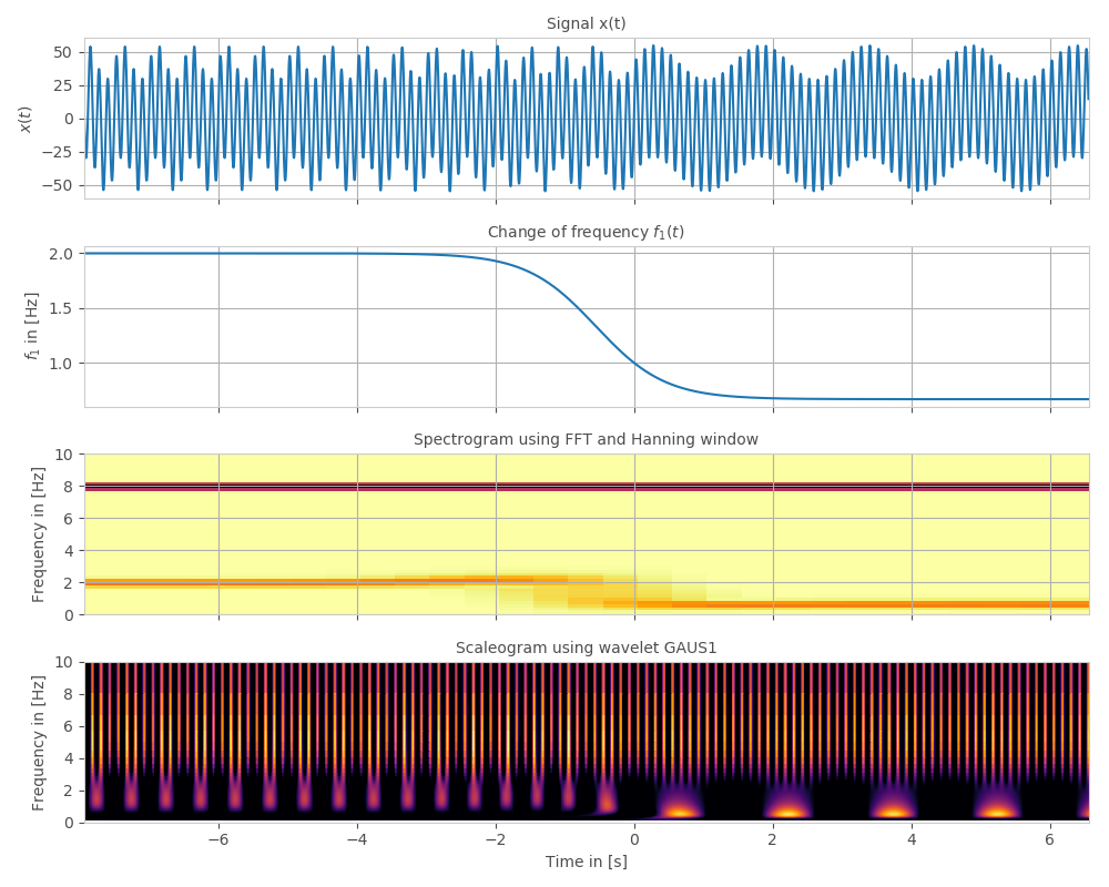
I am comparing FFT vs. CWT for a specific signal.

It is not clear to me how to read of the respective frequencies and amplitudes from the corresponding scaleogram of the CWT. Furthermore, I have the impression that the CWT is quite imprecise?

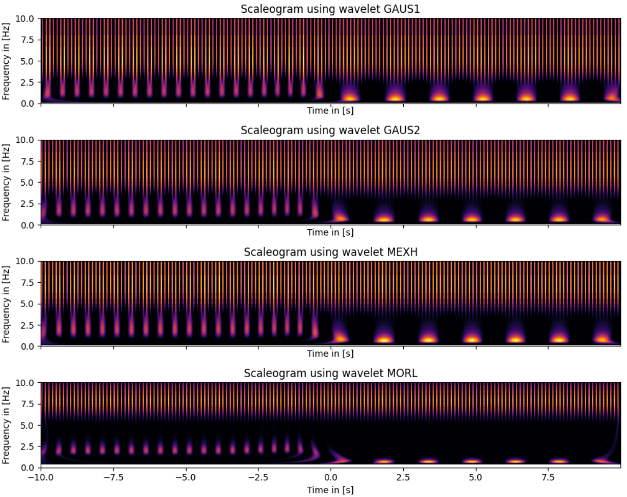
The spectrogram seems to be quite good in predicting the precise frequencies, but for the CWT, I tried many different wavelets and the result is the same.

Did I oversee something? Is this just not the appropriate tool for this problem?

Below, you find my example sourcecode and the corresponding plot.

import matplotlib.pyplot as plt
import numpy as np
from numpy import pi as π
from scipy.signal import spectrogram
import pywt

f_s = 200              # Sampling rate = number of measurements per second in [Hz]
t   = np.arange(-10,10, 1 / f_s) # Time between [-10s,10s].
T1  = np.tanh(t)/2  + 1.0 # Period in [s]
T2  = 0.125               # Period in [s]
f1  = 1 / T1              # Frequency in [Hz]
f2  = 1 / T2              # Frequency in [Hz] 

N = len(t)
x = 13 * np.sin(2 * π * f1 * t) + 42 * np.sin(2 * π * f2 * t)

fig, (ax1, ax2, ax3, ax4) = plt.subplots(4,1, sharex = True, figsize = (10,8))

# Signal
ax1.plot(t, x)
ax1.grid(True)
ax1.set_ylabel("$x(t)$")
ax1.set_title("Signal x(t)")

# Frequency change
ax2.plot(t, f1)
ax2.grid(True)
ax2.set_ylabel("$f_1$ in [Hz]")
ax2.set_title("Change of frequency $f_1(t)$")

# Moving fourier transform, i.e. spectrogram
Δt = 4 # window length in [s]
Nw = np.int(2**np.round(np.log2(Δt * f_s))) # Number of datapoints within window
f, t_, Sxx = spectrogram(x, f_s, window='hanning', nperseg=Nw, noverlap = Nw - 100, detrend=False, scaling='spectrum')
Δf  =  f[1] - f[0]
Δt_ = t_[1] - t_[0]
t2  = t_ + t[0] - Δt_

im = ax3.pcolormesh(t2, f - Δf/2, np.sqrt(2*Sxx), cmap = "inferno_r")#, alpha = 0.5)
ax3.grid(True)
ax3.set_ylabel("Frequency in [Hz]")
ax3.set_ylim(0, 10)
ax3.set_xlim(np.min(t2),np.max(t2))
ax3.set_title("Spectrogram using FFT and Hanning window")

# Wavelet transform, i.e. scaleogram
cwtmatr, freqs = pywt.cwt(x, np.arange(1, 512), "gaus1", sampling_period = 1 / f_s)
im2 = ax4.pcolormesh(t, freqs, cwtmatr, vmin=0, cmap = "inferno" )  
ax4.set_ylim(0,10)
ax4.set_ylabel("Frequency in [Hz]")
ax4.set_xlabel("Time in [s]")
ax4.set_title("Scaleogram using wavelet GAUS1")

# plt.savefig("./fourplot.pdf")

plt.show()

Pitchy

Answer 1

Your example waveform is composed of only a few pure tones at any given time, so the spectrogram plot is going to look very clean and readable.

The wavelet plot is going to look "messy" in comparison because you have to sum Gaussian wavelets of may different scales (and thus frequencies) to approximate each component pure tone in your original signal.

Both the short-time FFT and wavelet transforms are in the category time-frequency transforms, but have a different kernel. The kernel of the FFT is a pure tone, but the kernel of the wavelet transform you provided is a gaussian wavelet. The FFT pure tone kernel is going to cleanly correspond to the type of waveform you showed in your question, but the wavelet kernel will not.

I doubt that the result you got for different wavelets was numerically exactly the same. It probably just looks the same to the naked eye the way you've plotted it. It appears that you are using wavelets for the wrong purpose. Wavelets are more useful in analyzing the signal than plotting it. Wavelet analysis is unique as each datapoint in a wavelet composition encodes frequency, phase, and windowing information simultanesouly. This allows for designing algorithms that lie on a continuum between timeseries and frequency analysis, and can be very powerful.

As far as your claim about different wavelets giving the same results, this is clearly not true for all wavelets: I adapted your code, and it produces the image following it. Sure, GAUS2 and MEXH seem to produce similar plots (zoom in real close and you will find they are subtly different), but that's because the second-order gauss wavelet looks similar to the Mexican hat wavelet.

import matplotlib.pyplot as plt
import numpy as np
from numpy import pi as π
from scipy.signal import spectrogram, wavelets
import pywt
import random


f_s = 200              # Sampling rate = number of measurements per second in [Hz]
t   = np.arange(-10,10, 1 / f_s) # Time between [-10s,10s].
T1  = np.tanh(t)/2  + 1.0 # Period in [s]
T2  = 0.125               # Period in [s]
f1  = 1 / T1              # Frequency in [Hz]
f2  = 1 / T2              # Frequency in [Hz] 

N = len(t)
x = 13 * np.sin(2 * π * f1 * t) + 42 * np.sin(2 * π * f2 * t)

fig, (ax1, ax2, ax3, ax4) = plt.subplots(4,1, sharex = True, figsize = (10,8))


wvoptions=iter(['gaus1','gaus2','mexh','morl'])

axes=[ax1,ax2,ax3,ax4]


for ax in axes:
    # Wavelet transform, i.e. scaleogram
    try:
        choice=next(wvoptions)
        cwtmatr, freqs = pywt.cwt(x, np.arange(1, 512), choice, sampling_period = 1 / f_s)
        im = ax.pcolormesh(t, freqs, cwtmatr, vmin=0, cmap = "inferno" )  
        ax.set_ylim(0,10)
        ax.set_ylabel("Frequency in [Hz]")
        ax.set_xlabel("Time in [s]")
        ax.set_title(f"Scaleogram using wavelet {choice.upper()}")
    except:
        pass
# plt.savefig("./fourplot.pdf")

plt.tight_layout()
plt.show()

Subjoinder

Thanks for your answer, it goes in the right direction, but it is too vague to be useful yet. "I doubt that the result you got for different wavelets was numerically exactly the same." -- Try it out and plot it! If you can provide a convincing example for your statements and show exactly how the wavelet analysis is more useful than the FFT, I will believe you. Like this your answer only consists of a list of (most-likely correct) unproven statements. – Pitchy

@Pitchy please see my updated answer, also it will be unreasonable to code an entire example on wavelets being more useful than FFT. In fact, wavelet analysis is a new a new and growing field. Here is one paper that uses wavelets as features for ANN-based word recognition: researchgate.net/publication/…. Of course, FFT can also be used to produce these features, however wavelet analysis provides multi-resolution frequency analysis, which can be useful for isolating the most important features. You should research more on your own. – Subjoinder