Dear Crowd

Problem

I tried to calculate a spatial correlogram with the packages nfc, pgirmess, SpatialPack and spdep. However, I was troubling to define the start and end-point of the distance. I'm only interested in the spatial autocorrelation at smaller distances, but there on smaller bins. Additionally, as the raster is quite large (1.8 Megapixels), I run into memory troubles with these packages but the SpatialPack.

So I tried to produce my own code, using the function Moran from the package raster. But I must have some error, as the result for the complete dataset is somewhat different than the one from the other packages. If there is no error in my code, it might at least help others with similar problems.

Question

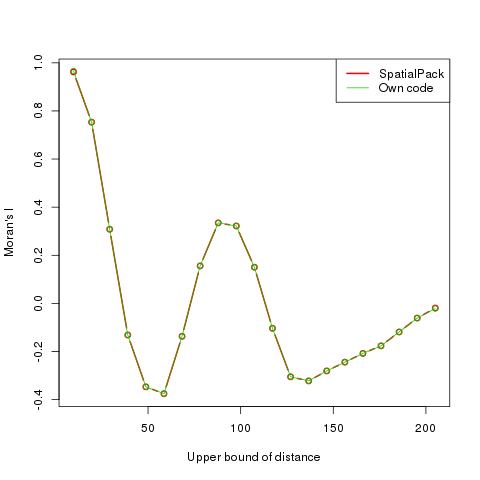
I'm not sure, whether my focal matrix is erroneous. Could you please tell me whether the central pixel needs to be incorporated? Using the testdata I can't show the differences between the methods, but on my complete dataset, there are differences visible, as shown in the Image below. However, the bins are not exactly the same (50m vs. 69m), so this might explain parts of the differences. However, at the first bin, this explanation seems not to be plausible to me. Or might the irregular shape of my raster, and different ways to handle NA's cause the difference?

Comparison of Own method with the one from SpatialPack

Runable Example

Testdata

The code for calculating the testdata is taken from http://www.petrkeil.com/?p=1050#comment-416317

# packages used for the data generation
library(raster)
library(vegan) # will be used for PCNM

# empty matrix and spatial coordinates of its cells
side=30
my.mat <- matrix(NA, nrow=side, ncol=side)
x.coord <- rep(1:side, each=side)*5
y.coord <- rep(1:side, times=side)*5
xy <- data.frame(x.coord, y.coord)

# all paiwise euclidean distances between the cells
xy.dist <- dist(xy)

# PCNM axes of the dist. matrix (from 'vegan' package)
pcnm.axes <- pcnm(xy.dist)$vectors

# using 8th PCNM axis as my atificial z variable
z.value <- pcnm.axes[,8]*200 + rnorm(side*side, 0, 1)

# plotting the artificial spatial data
r <- rasterFromXYZ(xyz = cbind(xy,z.value))
plot(r, axes=F)

Own Code

library(raster)
sp.Corr <- matrix(nrow = 0,ncol = 2)
formerBreak <- 0 #for the first run important
for (i in c(seq(10,200,10))) #Calculate the Morans I for these bins
{
  cat(paste0("..",i)) #print the bin, which is currently calculated
  w = focalWeight(r,d = i,type = 'circle')
  wTemp <- w #temporarily saves the weigtht matrix
  if (formerBreak>0) #if it is the second run
  {
    midpoint <- ceiling(ncol(w)/2) # get the midpoint      
    w[(midpoint-formerBreak):(midpoint+formerBreak),(midpoint-formerBreak):(midpoint+formerBreak)] <- w[(midpoint-formerBreak):(midpoint+formerBreak),(midpoint-formerBreak):(midpoint+formerBreak)]*(wOld==0)#set the previous focal weights to 0
    w <- w*(1/sum(w)) #normalizes the vector to sum the weights to 1
  }
  wOld <- wTemp #save this weight matrix for the next run
  mor <- Moran(r,w = w)
  sp.Corr <- rbind(sp.Corr,c(Moran =mor,Distance = i))
  formerBreak <- i/res(r)[1]#divides the breaks by the resolution of the raster to be able to translate them to the focal window
}
plot(x=sp.Corr[,2],y = sp.Corr[,1],type = "l",ylab = "Moran's I",xlab="Upper bound of distance")

Other methods to calculate the Spatial Correlogram

library(SpatialPack)
sp.Corr <- summary(modified.ttest(z.value,z.value,coords = xy,nclass = 21))
plot(x=sp.Corr$coef[,1],y = data$coef[,4],type = "l",ylab = "Moran's I",xlab="Upper bound of distance")

library(ncf)
ncf.cor <- correlog(x.coord, y.coord, z.value,increment=10, resamp=1)
plot(ncf.cor)

In order to compare the results of the correlogram, in your case, two things should be considered. (i) your code only works for bins proportional to the resolution of your raster. In that case, a bit of difference in the bins could make to include or exclude an important amount of pairs. (ii) The irregular shape of the raster has a strong impact of the pairs that are considered to compute the correlation for certain distance interval. So your code should deal with both, allow any value for the length of bin and consider the irregular shape of the raster. A small modification of your code to tackle those problems are below.

# SpatialPack correlation
library(SpatialPack)
test <- modified.ttest(z.value,z.value,coords = xy,nclass = 21)

# Own correlation
bins <- test$upper.bounds
library(raster)
sp.Corr <- matrix(nrow = 0,ncol = 2)
for (i in bins) {
  cat(paste0("..",i)) #print the bin, which is currently calculated
  w = focalWeight(r,d = i,type = 'circle')
  wTemp <- w #temporarily saves the weigtht matrix
  if (i > bins[1]) {
    midpoint <- ceiling(dim(w)/2) # get the midpoint      
    half_range <- floor(dim(wOld)/2)
    w[(midpoint[1] - half_range[1]):(midpoint[1] + half_range[1]),
      (midpoint[2] - half_range[2]):(midpoint[2] + half_range[2])] <- 
        w[(midpoint[1] - half_range[1]):(midpoint[1] + half_range[1]),
      (midpoint[2] - half_range[2]):(midpoint[2] + half_range[2])]*(wOld==0)
    w <- w * (1/sum(w)) #normalizes the vector to sum the weights to 1
  }
  wOld <- wTemp #save this weight matrix for the next run
  mor <- Moran(r,w=w)
  sp.Corr <- rbind(sp.Corr,c(Moran =mor,Distance = i))
}
# Comparing
plot(x=test$upper.bounds, test$imoran[,1], col = 2,type = "b",ylab = "Moran's I",xlab="Upper bound of distance", lwd = 2)
lines(x=sp.Corr[,2],y = sp.Corr[,1], col = 3)
points(x=sp.Corr[,2],y = sp.Corr[,1], col = 3)
legend('topright', legend = c('SpatialPack', 'Own code'), col = 2:3, lty = 1, lwd = 2:1)

The image shows that the results of using the SpatialPack package and the own code are the same.

Dear Crowd

Runable Example

Recommended topics

Hot tags