Obtain vertices of the ellipse on an ellipse covariance plot (created by `car::ellipse`)

Question

By following this post one can draw an ellipse with a given shape matrix (A):

library(car)
A <- matrix(c(20.43, -8.59,-8.59, 24.03), nrow = 2)
ellipse(c(-0.05, 0.09), shape=A, radius=1.44, col="red", lty=2, asp = 1)

Now how to get the major/minor (pair of intersect points of the major/minor axis and the ellipse) vertices of this ellipse?

Suzisuzie

I'm far unsure I'm understanding the Q, but x<-ellipse(..) will give a matrix of coordinates in x, isn't what you're after ? – Commiserate

@Tensibai. I want to get the pair of major (and minor) vertices out of all given vertices in x. – Suzisuzie

Do you mean the major and minor axes? – Rutheruthenia

Answer 1

For practical purposes, @Tensibai's answer is probably good enough. Just use a large enough value for the segments argument so that the points give a good approximation to the true vertices.

If you want something a bit more rigorous, you can solve for the location along the ellipse that maximises/minimises the distance from the center, parametrised by the angle. This is more complex than just taking angle={0, pi/2, pi, 3pi/2} because of the presence of the shape matrix. But it's not too difficult:

# location along the ellipse
# linear algebra lifted from the code for ellipse()
ellipse.loc <- function(theta, center, shape, radius)
{
    vert <- cbind(cos(theta), sin(theta))
    Q <- chol(shape, pivot=TRUE)
    ord <- order(attr(Q, "pivot"))
    t(center + radius*t(vert %*% Q[, ord]))
}

# distance from this location on the ellipse to the center 
ellipse.rad <- function(theta, center, shape, radius)
{
    loc <- ellipse.loc(theta, center, shape, radius)
    (loc[,1] - center[1])^2 + (loc[,2] - center[2])^2
}

# ellipse parameters
center <- c(-0.05, 0.09)
A <- matrix(c(20.43, -8.59, -8.59, 24.03), nrow=2)
radius <- 1.44

# solve for the maximum distance in one hemisphere (hemi-ellipse?)
t1 <- optimize(ellipse.rad, c(0, pi - 1e-5), center=center, shape=A, radius=radius, maximum=TRUE)$m
l1 <- ellipse.loc(t1, center, A, radius)

# solve for the minimum distance
t2 <- optimize(ellipse.rad, c(0, pi - 1e-5), center=center, shape=A, radius=radius)$m
l2 <- ellipse.loc(t2, center, A, radius)

# other points obtained by symmetry
t3 <- pi + t1
l3 <- ellipse.loc(t3, center, A, radius)

t4 <- pi + t2
l4 <- ellipse.loc(t4, center, A, radius)

# plot everything
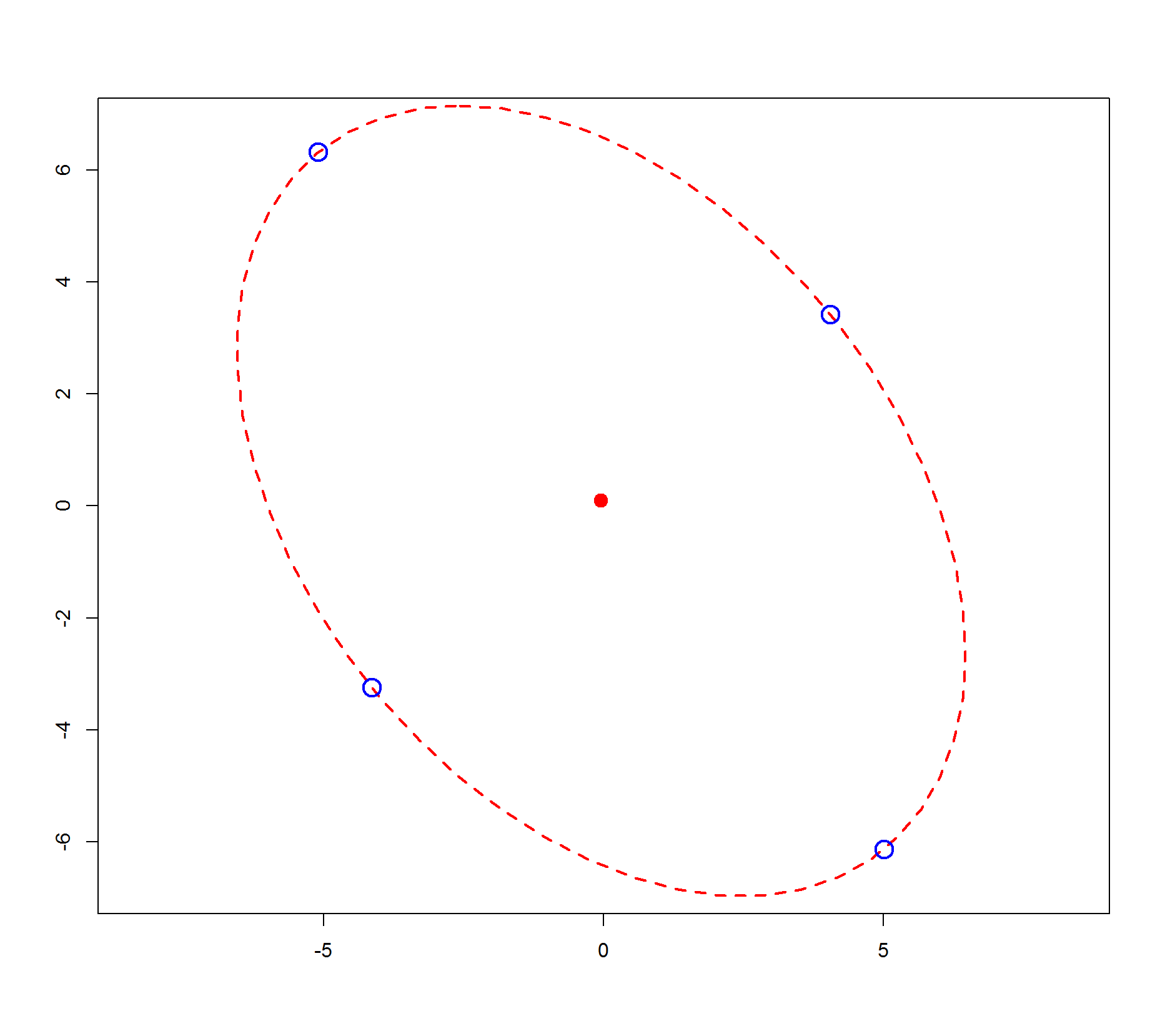
MASS::eqscplot(center[1], center[2], xlim=c(-7, 7), ylim=c(-7, 7), xlab="", ylab="")
ellipse(center, A, radius, col="red", lty=2)
points(rbind(l1, l2, l3, l4), cex=2, col="blue", lwd=2)

Rutheruthenia

A fully rigorous solution would be to find the locations of the minima/maxima from first principles, rather than numerically. But I've forgotten all my mathematics of conic sections. – Rutheruthenia

Nice approach :) I've the same problem with the conic sections maths, they're too far away. – Commiserate

Thanks @Hong Ooi. From plot it looks it is perfect. It solve my problem. – Suzisuzie

Answer 2

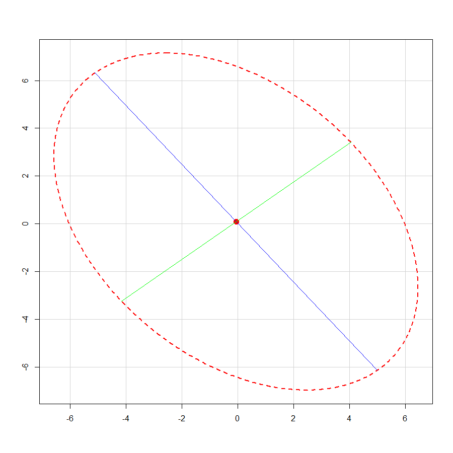
I know this question has been seen as solved, but actually there is a super elegant solution to this, in only a few lines as follow. Such computation is precise, without any sort of numerical optimization.

## target covariance matrix
A <- matrix(c(20.43, -8.59,-8.59, 24.03), nrow = 2)

E <- eigen(A, symmetric = TRUE)  ## symmetric eigen decomposition
U <- E[[2]]  ## eigen vectors, i.e., rotation matrix
D <- sqrt(E[[1]])  ## root eigen values, i.e., scaling factor

r <- 1.44  ## radius of original circle
Z <- rbind(c(r, 0), c(0, r), c(-r, 0), c(0, -r))  ## original vertices on major / minor axes
Z <- tcrossprod(Z * rep(D, each = 4), U)  ## transformed vertices on major / minor axes

#          [,1]      [,2]
#[1,] -5.055136  6.224212
#[2,] -4.099908 -3.329834
#[3,]  5.055136 -6.224212
#[4,]  4.099908  3.329834

C0 <- c(-0.05, 0.09)  ## new centre
Z <- Z + rep(C0, each = 4)  ## shift to new centre

#          [,1]      [,2]
#[1,] -5.105136  6.314212
#[2,] -4.149908 -3.239834
#[3,]  5.005136 -6.134212
#[4,]  4.049908  3.419834

In order to explain the mathematics behind, I am going to take 3 steps:

1. Where does this Ellipse come from?
2. Cholesky decomposition method and its drawback.
3. Eigen decomposition method and its natural interpretation.

---

Where does this ellipse comes from?

In practice, this ellipse can be obtained by some linear transformation to the unit circle x ^ 2 + y ^ 2 = 1.

---

Cholesky decomposition method and its drawback

## initial circle
r <- 1.44
theta <- seq(0, 2 * pi, by = 0.01 * pi)
X <- r * cbind(cos(theta), sin(theta))

## target covariance matrix
A <- matrix(c(20.43, -8.59,-8.59, 24.03), nrow = 2)

R <- chol(A)  ## Cholesky decomposition
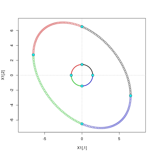
X1 <- X %*% R  ## linear transformation

Z <- rbind(c(r, 0), c(0, r), c(-r, 0), c(0, -r))  ## original vertices on major / minor axes
Z1 <- Z %*% R  ## transformed coordinates

## different colour per quadrant
g <- floor(4 * (1:nrow(X) - 1) / nrow(X)) + 1

## draw ellipse
plot(X1, asp = 1, col = g)
points(Z1, cex = 1.5, pch = 21, bg = 5)

## draw circle
points(X, col = g, cex = 0.25)
points(Z, cex = 1.5, pch = 21, bg = 5)

## draw axes
abline(h = 0, lty = 3, col = "gray", lwd = 1.5)
abline(v = 0, lty = 3, col = "gray", lwd = 1.5)

We see that the linear transform matrix R does not appear to have natural interpretation. The original vertices of the circle do not map to vertices of the ellipse.

---

Eigen decomposition method and its natural interpretation

## initial circle
r <- 1.44
theta <- seq(0, 2 * pi, by = 0.01 * pi)
X <- r * cbind(cos(theta), sin(theta))

## target covariance matrix
A <- matrix(c(20.43, -8.59,-8.59, 24.03), nrow = 2)

E <- eigen(A, symmetric = TRUE)  ## symmetric eigen decomposition
U <- E[[2]]  ## eigen vectors, i.e., rotation matrix
D <- sqrt(E[[1]])  ## root eigen values, i.e., scaling factor

r <- 1.44  ## radius of original circle
Z <- rbind(c(r, 0), c(0, r), c(-r, 0), c(0, -r))  ## original vertices on major / minor axes

## step 1: re-scaling
X1 <- X * rep(D, each = nrow(X))  ## anisotropic expansion to get an axes-aligned ellipse
Z1 <- Z * rep(D, each = 4L)  ## vertices on axes

## step 2: rotation
Z2 <- tcrossprod(Z1, U)  ## rotated vertices on major / minor axes
X2 <- tcrossprod(X1, U)  ## rotated ellipse

## different colour per quadrant
g <- floor(4 * (1:nrow(X) - 1) / nrow(X)) + 1

## draw rotated ellipse and vertices
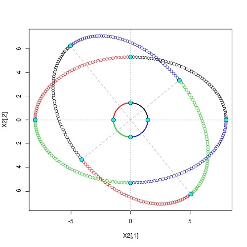
plot(X2, asp = 1, col = g)
points(Z2, cex = 1.5, pch = 21, bg = 5)

## draw axes-aligned ellipse and vertices
points(X1, col = g)
points(Z1, cex = 1.5, pch = 21, bg = 5)

## draw original circle
points(X, col = g, cex = 0.25)
points(Z, cex = 1.5, pch = 21, bg = 5)

## draw axes
abline(h = 0, lty = 3, col = "gray", lwd = 1.5)
abline(v = 0, lty = 3, col = "gray", lwd = 1.5)

## draw major / minor axes
segments(Z2[1,1], Z2[1,2], Z2[3,1], Z2[3,2], lty = 2, col = "gray", lwd = 1.5)
segments(Z2[2,1], Z2[2,2], Z2[4,1], Z2[4,2], lty = 2, col = "gray", lwd = 1.5)

Here we see that in both stages of the transform, vertices are still mapped to vertices. It is exactly based on such property we have the neat solution given at the very beginning.

Gasteropod

I was looking for this answer, extremely well explained, great job! – Hustings

Wow..that's great. Thank you for such a great effort. – Suzisuzie

Sorry what is a "vertex" of a circle? I thought vertex is a point where two or more lines or edges meet, but circle has only one line and no edges? And what do you mean by "vertices are still mapped to vertices" in the last sentence of your answer? Thank you – Shrivel

Answer 3

Still highly unsure this will really answer the question but here's my try:

first, define the center of the ellipse as a vector for later use:

center<-c(x=-0.05, y=0.09)

draw the ellipse and get the matrix of "points" with enought values to get a close enough to reality point:

tmp<-ellipse(c(-0.05, 0.09), shape=A, radius=1.44, segments=1e3, col="red", lty=2,add=FALSE)

Create a data.table with it and compute the distance of each point toward center (point_x - center_x)² + (point_y - center_y)²:

dt <- data.table(tmp)
dt[,dist:={dx=x-center[1];dy=y-center[2];dx*dx+dy*dy}]

Order the vertices by distance:

setorder(dt,dist)

Get the min and max points:

> tail(dt,2)
           x         y     dist
1:  4.990415 -6.138039 64.29517
2: -5.110415  6.318039 64.29517
> head(dt,2)
       x        y     dist
1:  4.045722  3.41267 27.89709
2: -4.165722 -3.23267 27.89709

Don't add too much segments or the two first values will be two points really close to each other instead of opposite.

with a visual results this sounds not so exact at end:

Commiserate

Thanks for your answer. I have plotted the major axes from the from your given vertices and observed that the line is missing the origin. The major vertices should pass through the center. – Suzisuzie

Unsure, but taking only 1 and using it's exact opposite should do, I'll try and update answer accordingly after lunch – Commiserate

I took one of the point from two points of the major vertices (which has max distance from the center) and draw the line which pass through the center and the maximum distance major vertex. This can be thought as the major axes. But it seems from the plot that this axes is not bisecting the ellipse symmetrically. – Suzisuzie

@Suzisuzie That's my main concern, the points returned by ellipse are to draw the 'ticks'. I'll play with it to see if I can get something smoother and find a better point. I'm unsure of how the ellipse formula can be expressed at end, so it's hard to reverse it to get the real 'nearest point' (at float precision difference) – Commiserate