Iteratively fitting polynomial curve

Question

I want to iteratively fit a curve to data in python with the following approach:

1. Fit a polynomial curve (or any non-linear approach)
2. Discard values > 2 standard deviation from mean of the curve
3. repeat steps 1 and 2 till all values are within confidence interval of the curve

I can fit a polynomial curve as follows:

vals = array([0.00441025, 0.0049001 , 0.01041189, 0.47368389, 0.34841961,
       0.3487533 , 0.35067096, 0.31142986, 0.3268407 , 0.38099566,
       0.3933048 , 0.3479948 , 0.02359819, 0.36329588, 0.42535543,
       0.01308297, 0.53873956, 0.6511364 , 0.61865282, 0.64750302,
       0.6630047 , 0.66744816, 0.71759617, 0.05965622, 0.71335208,
       0.71992683, 0.61635697, 0.12985441, 0.73410642, 0.77318621,
       0.75675988, 0.03003641, 0.77527201, 0.78673995, 0.05049178,
       0.55139476, 0.02665514, 0.61664748, 0.81121749, 0.05521697,
       0.63404375, 0.32649395, 0.36828268, 0.68981099, 0.02874863,
       0.61574739])
x_values = np.linspace(0, 1, len(vals))
poly_degree = 3

coeffs = np.polyfit(x_values, vals, poly_degree)
poly_eqn = np.poly1d(coeffs)
y_hat = poly_eqn(x_values)

How do I do steps 2 and 3?

Iapetus

you only used python & numpy tags, are you open to using other python packages like scipy, sklearn, etc.? – Uncover

@JohnE, absolutely, anything Python is fine – Iapetus

can you explain a little more about your second part? specially about mean of curve. – Motivation

Answer 1

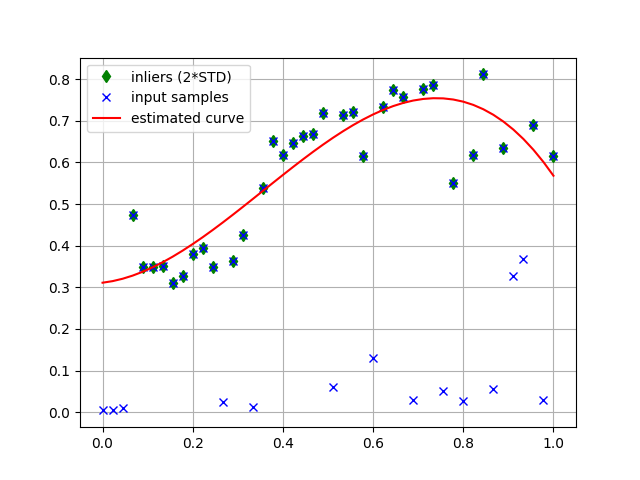
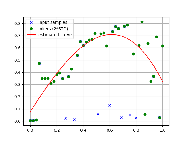
With the eliminating points too far from an expected solution, you are probably looking for RANSAC (RANdom SAmple Consensus), which is fitting a curve (or any other function) to data within certain bounds, like your case with 2*STD.

You can use scikit-learn RANSAC estimator which is well aligned with included regressors such as LinearRegression. For your polynomial case you need to define your own regression class:

from sklearn.metrics import mean_squared_error
class PolynomialRegression(object):
    def __init__(self, degree=3, coeffs=None):
        self.degree = degree
        self.coeffs = coeffs

    def fit(self, X, y):
        self.coeffs = np.polyfit(X.ravel(), y, self.degree)

    def get_params(self, deep=False):
        return {'coeffs': self.coeffs}

    def set_params(self, coeffs=None, random_state=None):
        self.coeffs = coeffs

    def predict(self, X):
        poly_eqn = np.poly1d(self.coeffs)
        y_hat = poly_eqn(X.ravel())
        return y_hat

    def score(self, X, y):
        return mean_squared_error(y, self.predict(X))

and then you can use RANSAC

from sklearn.linear_model import RANSACRegressor
ransac = RANSACRegressor(PolynomialRegression(degree=poly_degree),
                         residual_threshold=2 * np.std(y_vals),
                         random_state=0)
ransac.fit(np.expand_dims(x_vals, axis=1), y_vals)
inlier_mask = ransac.inlier_mask_

Note, the X variable is transformed to 2d array as it is required by sklearn RANSAC implementation and in our custom class flatten back because of numpy polyfit function works with 1d array.

y_hat = ransac.predict(np.expand_dims(x_vals, axis=1))
plt.plot(x_vals, y_vals, 'bx', label='input samples')
plt.plot(x_vals[inlier_mask], y_vals[inlier_mask], 'go', label='inliers (2*STD)')
plt.plot(x_vals, y_hat, 'r-', label='estimated curve')

moreover, playing with the polynomial order and residual distance I got following results with degree=4 and range 1*STD

Another option is to use higher order regressor like Gaussian process

from sklearn.gaussian_process import GaussianProcessRegressor
ransac = RANSACRegressor(GaussianProcessRegressor(),
                         residual_threshold=np.std(y_vals))

Talking about generalization to DataFrame, you just need to set that all columns except one are features and the one remaining is the output, like here:

import pandas as pd
df = pd.DataFrame(np.array([x_vals, y_vals]).T)
ransac.fit(df[df.columns[:-1]], df[df.columns[-1]])
y_hat = ransac.predict(df[df.columns[:-1]])

Excitor

thanks @Excitor B.! Do you know if it is possible to ignore the negative outliers completely? – Iapetus

what do you mean by negative outliers? in general, outliers are points too far from expectation and the distance is always positive... – Excitor

Answer 2

it doesn't look like you'll get anything worthwhile following that procedure, there are much better techniques for handling unexpected data. googling for "outlier detection" would be a good start.

with that said, here's how to answer your question:

start by pulling in libraries and getting some data:

import matplotlib.pyplot as plt
import numpy as np

Y = np.array([
    0.00441025, 0.0049001 , 0.01041189, 0.47368389, 0.34841961,
    0.3487533 , 0.35067096, 0.31142986, 0.3268407 , 0.38099566,
    0.3933048 , 0.3479948 , 0.02359819, 0.36329588, 0.42535543,
    0.01308297, 0.53873956, 0.6511364 , 0.61865282, 0.64750302,
    0.6630047 , 0.66744816, 0.71759617, 0.05965622, 0.71335208,
    0.71992683, 0.61635697, 0.12985441, 0.73410642, 0.77318621,
    0.75675988, 0.03003641, 0.77527201, 0.78673995, 0.05049178,
    0.55139476, 0.02665514, 0.61664748, 0.81121749, 0.05521697,
    0.63404375, 0.32649395, 0.36828268, 0.68981099, 0.02874863,
    0.61574739])
X = np.linspace(0, 1, len(Y))

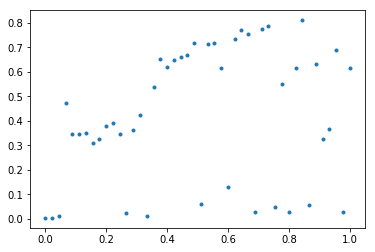
next do an initial plot of the data:

plt.plot(X, Y, '.')

as this lets you see what we're dealing with and whether a polynomial would ever be a good fit --- short answer is that this method isn't going to get very far with this sort of data

at this point we should stop, but to answer the question I'll go on, mostly following your polynomial fitting code:

poly_degree = 5
sd_cutoff = 1 # 2 keeps everything

coeffs = np.polyfit(X, Y, poly_degree)
poly_eqn = np.poly1d(coeffs)

Y_hat = poly_eqn(X)
delta = Y - Y_hat
sd_p = np.std(delta)

ok = abs(delta) < sd_p * sd_cutoff

hopefully this makes sense, I use a higher degree polynomial and only cutoff at 1SD because otherwise nothing will be thrown away. the ok array contains True values for those points that are within sd_cutoff standard deviations

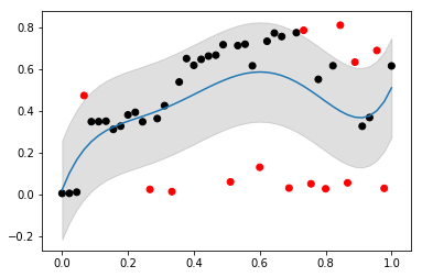
to check this, I'd then do another plot. something like:

plt.scatter(X, Y, color=np.where(ok, 'k', 'r'))
plt.fill_between(
    X,
    Y_hat - sd_p * sd_cutoff, 
    Y_hat + sd_p * sd_cutoff,
    color='#00000020')
plt.plot(X, Y_hat)

which gives me:

so the black dots are the points to keep (i.e. X[ok] gives me these back, and np.where(ok) gives you indicies).

you can play around with the parameters, but you probably want a distribution with fatter tails (e.g. a Student's T-distribution) but, as I said above, using Google for outlier detection would be my suggestion

Boardman

I do not see how you implemented the point 3 with alternating fitting and section... – Excitor

@JirkaB. using a "cutoff" of 2SDs wouldn't actually remove anything, hence my "2 keeps everything" comment and not actually implementing the loop. I've just noticed the OP's comment that "smoothing approach can be something more robust", and your RANSAC suggestion would be a good option here. I've been playing with a Bayesian Gaussian Process MCMC approach as another alternative, but it's a few hundred lines of code and not sure if it's worth posting. maybe as another answer as it might be interesting to other people – Boardman

you can even integrated Bayesian Gaussian Process regression inside RANSAC – Excitor

you can certainly put a GP in RANSAC. To call it Bayesian I'd want to be integrating over all parameter uncertainty, the scikit implementation just seems to optimise hyper-parameters and ignores any uncertainty. If you just want a single point estimate then this is of course fine, I just prefer to be more honest about uncertainty – Boardman

that sounds promising... another way could be ProSAC - researchgate.net/publication/4156175 – Excitor

Answer 3

There are three functions need to solve this. First a line fitting function is necesary to fit a line to a set of points:

def fit_line(x_values, vals, poly_degree):
    coeffs = np.polyfit(x_values, vals, poly_degree)
    poly_eqn = np.poly1d(coeffs)
    y_hat = poly_eqn(x_values)
    return poly_eqn, y_hat

We need to know the standard deviation from the points to the line. This function computes that standard deviation:

def compute_sd(x_values, vals, y_hat):
    distances = []
    for x,y, y1 in zip(x_values, vals, y_hat): distances.append(abs(y - y1))
    return np.std(distances)

Finally, we need to compare the distance from a point to the line. The point needs to be thrown out if the distance from the point to the line is greater than two times the standard deviation.

def compare_distances(x_values, vals):    
    new_vals, new_x_vals = [],[]
    for x,y in zip(x_values, vals):    
        y1 = np.polyval(poly_eqn, x)
        distance = abs(y - y1)
        if distance < 2*sd:
            plt.plot((x,x),(y,y1), c='g')
            new_vals.append(y)
            new_x_vals.append(x)
        else:
            plt.plot((x,x),(y,y1), c='r')
            plt.scatter(x,y, c='r')
    return new_vals, new_x_vals

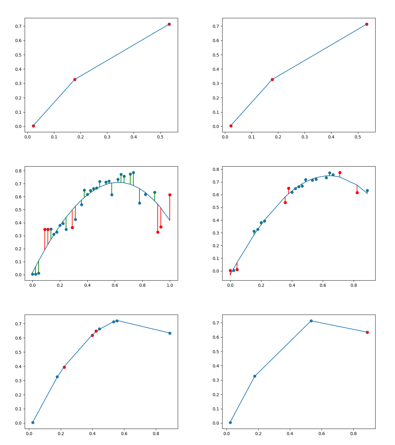
As you can see in the following graphs, this method does not work well for fitting a line to data that has a lot of outliers. All the points end up getting eliminated for being too far from the fitted line.

while len(vals)>0:
    poly_eqn, y_hat = fit_line(x_values, vals, poly_degree)
    plt.scatter(x_values, vals)
    plt.plot(x_values, y_hat)
    sd = compute_sd(x_values, vals, y_hat)
    new_vals, new_x_vals = compare_distances(x_values, vals)
    plt.show()
    vals, x_values = np.array(new_vals), np.array(new_x_vals)

Bula