Asked 17/1 at 2:16 Answered 24/1 at 14:52

Solved r algorithm performance random-walk

I have the following situation:

A variable moves +1 with prob=0.5 and -1 with prob=-0.5 ... if this Markov Chain starts at position=5

Situation 1: What is the expected time at which the variable will first reach position = 0?
Situation 2: What is the expected time at which the variable will first reach position= 0 AFTER having gone to position=10 at least once?

I tried to do this as follows (I created a tracking variable to see where the simulation gets stuck):

# the simulations can take a long time to run, I interrupted them

library(ggplot2)
library(gridExtra)

n_sims <- 100
times_to_end_0 <- numeric(n_sims)
times_to_end_0_after_10 <- numeric(n_sims)
paths_0 <- vector("list", n_sims)
paths_0_after_10 <- vector("list", n_sims)

for (i in 1:n_sims) {
    print(paste("Running simulation", i, "for situation 1..."))
    y <- 5
    time <- 0
    path_0 <- c(y)

    while(y > 0) {
        step <- sample(c(-1, 1), 1, prob = c(0.5, 0.5))
        y <- y + step
        path_0 <- c(path_0, y)
        time <- time + 1

        if (y == 0) {
            times_to_end_0[i] <- time
            paths_0[[i]] <- data.frame(time = 1:length(path_0), y = path_0, sim = i)
            break
        }
    }

    print(paste("Running simulation", i, "for situation 2..."))
    y <- 5
    time <- 0
    reached_10 <- FALSE
    path_0_after_10 <- c(y)

    while(y > 0 || !reached_10) {
        step <- sample(c(-1, 1), 1, prob = c(0.5, 0.5))
        y <- y + step
        path_0_after_10 <- c(path_0_after_10, y)
        time <- time + 1

        if (y == 10) {
            reached_10 <- TRUE
        }

        if (y == 0 && reached_10) {
            times_to_end_0_after_10[i] <- time
            paths_0_after_10[[i]] <- data.frame(time = 1:length(path_0_after_10), y = path_0_after_10, sim = i)
            break
        }
    }
}

df1 <- data.frame(time = times_to_end_0)
df2 <- data.frame(time = times_to_end_0_after_10[times_to_end_0_after_10 > 0])

mean1 <- mean(log(df1$time))
mean2 <- mean(log(df2$time))

p1 <- ggplot(df1, aes(x = log(time))) +
    geom_density() +
    geom_vline(aes(xintercept = exp(mean1)), color = "red", linetype = "dotted") +
    labs(title = paste("Density of Times to Reach 0 - Mean Time:", round(exp(mean1), 2)), x = "Time", y = "Density") + theme_bw()

p2 <- ggplot(df2, aes(x = log(time))) +
    geom_density() +
    geom_vline(aes(xintercept = exp(mean2)), color = "red", linetype = "dotted") +
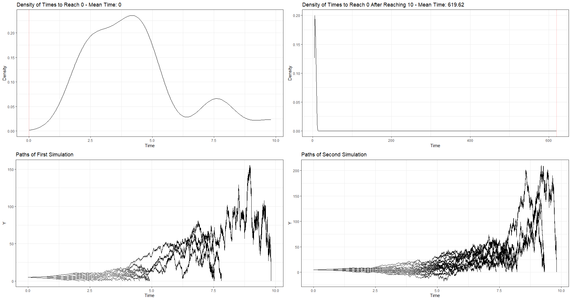
    labs(title = paste("Density of Times to Reach 0 After Reaching 10 - Mean Time:", round(exp(mean2), 2)), x = "Time", y = "Density") + theme_bw() 

plot_df_0 <- do.call(rbind, paths_0)

p3 <- ggplot(plot_df_0, aes(x = log(time), y = y, group = sim)) +
    geom_line() +
    labs(title = "Paths of First Simulation", x = "Time", y = "Y") +
    theme_bw()

plot_df_0_after_10 <- do.call(rbind, paths_0_after_10)

p4 <- ggplot(plot_df_0_after_10, aes(x = log(time), y = y, group = sim)) +
    geom_line() +
    labs(title = "Paths of Second Simulation", x = "Time", y = "Y") +
    theme_bw()

grid.arrange(p1, p2, p3, p4, ncol = 2)

My Question: Is there anything I can do to improve the efficiency of this simulation?

Thanks!

Concatenate answered 17/1 at 2:16 Comment(0)

Calling sample() in each cycle of your for/while loop creates a lot of overhead and causes your simulations to run slow.

The solution below runs sample() once per simulation with a size of 1e6 (1,000,000). You could also go bigger, 1e7 seems reasonably fast on my machine and all cycles have hit 0 for several runs with 1e7. At 1e8 things get slow and at 1e9 is likely too much for most machines. The smaller you set the sample size the more runs that don’t hit 0 you’ll get.

Function

This function relies on vectorization to speed things up.

sim <- function(y = 5,
                size = 1e6) {
  steps <- sample(c(-1, 1),
                  size,
                  prob = c(0.5, 0.5),
                  replace = TRUE)
  y_steps <- c(y, steps)
  y_steps_cum <- cumsum(y_steps)
  times <- which(y_steps_cum == 0)
  times_to_0 <- times[1]
  path <- if (!is.na(times_to_0))
    y_steps_cum[1:times_to_0]
  else
    NA
  touched_10 <- which(y_steps_cum == 10)[1]
  times_to_0_after_10 <-
    if (!is.na(touched_10))
      times[times > touched_10][1]
  else
    NA
  path_to_0_after_10 <-
    if (!is.na(times_to_0_after_10))
      y_steps_cum[1:times_to_0_after_10]
  else
    NA
  
  list(
    times_to_0 = times_to_0,
    path = list(path),
    touched_10 = touched_10,
    times_to_0_after_10 = times_to_0_after_10,
    path_to_0_after_10 = list(path_to_0_after_10)
  )
}

A single simulation:

sim()
#> $times_to_0
#> [1] 314
#> 
#> $path
#> $path[[1]]
#>   [1]  5  4  3  2  3  4  3  4  3  2  3  4  5  6  7  8  9  8  9 10  9 10  9  8  7
#>  [26]  6  7  6  5  4  5  6  7  8  9 10  9 10 11 12 11 12 11 12 13 12 11 12 13 12
#>  [51] 13 12 11 12 11 10 11 10 11 10 11 12 13 12 13 14 13 12 11 10  9  8  7  6  7
#>  [76]  6  7  8  9  8  7  8  9  8  7  8  7  6  7  8  9  8  9  8  7  6  5  6  5  4
#> [101]  3  4  5  6  5  6  5  6  7  8  7  8  7  6  7  6  7  8  9  8  7  8  9  8  9
#> [126]  8  7  6  5  6  7  8  9  8  7  8  7  8  9 10  9 10  9  8  9  8  9  8  9 10
#> [151] 11 12 11 12 11 10 11 10 11 12 11 12 13 12 13 14 15 16 15 14 15 14 13 12 13
#> [176] 14 15 14 15 16 17 18 19 18 19 20 19 18 17 16 15 14 13 12 11 10 11 10  9 10
#> [201]  9 10 11 12 11 10 11 10  9 10 11 10 11 12 13 12 13 14 15 14 15 16 17 16 15
#> [226] 14 15 14 13 12 11 10  9  8  9  8  7  8  9 10 11 10 11 12 11 10 11 10  9 10
#> [251]  9 10 11 12 11 12 11 10  9 10 11 12 11 12 13 12 11 12 13 12 13 14 13 12 13
#> [276] 12 11 12 11 10  9  8  7  6  7  8  7  6  7  6  5  6  5  4  5  4  3  2  3  4
#> [301]  5  4  5  4  5  4  5  4  3  2  1  2  1  0
#> 
#> 
#> $touched_10
#> [1] 20
#> 
#> $times_to_0_after_10
#> [1] 314
#> 
#> $path_to_0_after_10
#> $path_to_0_after_10[[1]]
#>   [1]  5  4  3  2  3  4  3  4  3  2  3  4  5  6  7  8  9  8  9 10  9 10  9  8  7
#>  [26]  6  7  6  5  4  5  6  7  8  9 10  9 10 11 12 11 12 11 12 13 12 11 12 13 12
#>  [51] 13 12 11 12 11 10 11 10 11 10 11 12 13 12 13 14 13 12 11 10  9  8  7  6  7
#>  [76]  6  7  8  9  8  7  8  9  8  7  8  7  6  7  8  9  8  9  8  7  6  5  6  5  4
#> [101]  3  4  5  6  5  6  5  6  7  8  7  8  7  6  7  6  7  8  9  8  7  8  9  8  9
#> [126]  8  7  6  5  6  7  8  9  8  7  8  7  8  9 10  9 10  9  8  9  8  9  8  9 10
#> [151] 11 12 11 12 11 10 11 10 11 12 11 12 13 12 13 14 15 16 15 14 15 14 13 12 13
#> [176] 14 15 14 15 16 17 18 19 18 19 20 19 18 17 16 15 14 13 12 11 10 11 10  9 10
#> [201]  9 10 11 12 11 10 11 10  9 10 11 10 11 12 13 12 13 14 15 14 15 16 17 16 15
#> [226] 14 15 14 13 12 11 10  9  8  9  8  7  8  9 10 11 10 11 12 11 10 11 10  9 10
#> [251]  9 10 11 12 11 12 11 10  9 10 11 12 11 12 13 12 11 12 13 12 13 14 13 12 13
#> [276] 12 11 12 11 10  9  8  7  6  7  8  7  6  7  6  5  6  5  4  5  4  3  2  3  4
#> [301]  5  4  5  4  5  4  5  4  3  2  1  2  1  0

100 simulations:

library(tidyverse)

tictoc::tic() # tic() and toc() are for benchmarking

res <-
  lapply(rep(5, 100),
         sim) |>
  bind_rows(.id = "sim")

tictoc::toc()
#> 2.596 sec elapsed

res
#> # A tibble: 100 × 6
#>    sim   times_to_0 path       touched_10 times_to_0_after_10 path_to_0_after_10
#>    <chr>      <int> <list>          <int>               <int> <list>            
#>  1 1           3202 <dbl>              26                3202 <dbl [3,202]>     
#>  2 2           1690 <dbl>              16                1690 <dbl [1,690]>     
#>  3 3             32 <dbl [32]>      11586               12012 <dbl [12,012]>    
#>  4 4            386 <dbl>              54                 386 <dbl [386]>       
#>  5 5            280 <dbl>              20                 280 <dbl [280]>       
#>  6 6             20 <dbl [20]>        272                2890 <dbl [2,890]>     
#>  7 7           3520 <dbl>              20                3520 <dbl [3,520]>     
#>  8 8            160 <dbl>               8                 160 <dbl [160]>       
#>  9 9         141814 <dbl>               8              141814 <dbl [141,814]>   
#> 10 10          1474 <dbl>              10                1474 <dbl [1,474]>     
#> # ℹ 90 more rows

Plotting Results

library(ggplot2)
library(gridExtra)
#> 
#> Attaching package: 'gridExtra'
#> The following object is masked from 'package:dplyr':
#> 
#>     combine

mean1 <- mean(log(res$times_to_0), na.rm = TRUE)
mean2 <- mean(log(res$times_to_0_after_10), na.rm = TRUE)

p1 <-
  ggplot(res, aes(x = log(times_to_0))) +
  geom_density() +
  geom_vline(aes(xintercept = exp(mean1)),
             color = "red",
             linetype = "dotted") +
  labs(
    title = paste("Density of Times to Reach 0 - Mean Time:", round(exp(mean1), 2)),
    x = "Time",
    y = "Density"
  ) + theme_bw()

p2 <- 
  ggplot(res, aes(x = log(times_to_0_after_10))) +
  geom_density() +
  geom_vline(aes(xintercept = exp(mean2)),
             color = "red",
             linetype = "dotted") +
  labs(
    title = paste(
      "Density of Times to Reach 0 After Reaching 10 - Mean Time:",
      round(exp(mean2), 2)
    ),
    x = "Time",
    y = "Density"
  ) + theme_bw()

p3 <-
  res |>
  select(sim, path) |>
  unnest(path) |>
  mutate(time = 1:n(), .by = sim) |>
  ggplot(aes(
    x = log(time),
    y = path,
    group = sim
  )) +
  geom_line(linewidth = .05) +
  labs(title = "Paths of First Simulation", x = "Time", y = "Y") +
  theme_bw()

p4 <-
  res |>
  select(sim, path_to_0_after_10) |>
  unnest(path_to_0_after_10) |>
  mutate(time = 1:n(), .by = sim) |>
  ggplot(aes(
    x = log(time),
    y = path_to_0_after_10,
    group = sim
  )) +
  geom_line(linewidth = .05) +
  labs(title = "Paths of Second Simulation", x = "Time", y = "Y") +
  theme_bw()

grid.arrange(p1, p2, p3, p4, ncol = 2)
#> Warning: Removed 1 rows containing non-finite values (`stat_density()`).
#> Warning: Removed 3 rows containing non-finite values (`stat_density()`).
#> Warning: Removed 1 row containing missing values (`geom_line()`).
#> Warning: Removed 3 rows containing missing values (`geom_line()`).

Espinosa answered 17/1 at 4:35 Comment(1)

@ Till: thank you so much for this wonderful answer! – Concatenate 19/1 at 13:53

It is well known that the expected time to move from k to k + 1 in a symmetric random walk is infinite. We can still simulate right-censored walk times.

Below is a more direct approach to the simulation. Think about moving from 5 to 6. It will always take an odd number of steps. The probability of it taking 2*n - 1 steps is abs(choose(0.5, n)). Once it reaches 6, the number of steps to go from 6 to 7 is independent of the number of steps it took to go from 5 to 6.

To speed up the simulation, first pre-calculate the CDF of the number of steps to move 1 space. If we want to simulate how many steps it takes to move n spaces total, we can sum n random samples from the pre-calculated CDF. (The distribution is very heavy tailed, so we will let it run up to a maximum number of steps, at which the simulation will be terminated early and return Inf.)

Implementing the simulation as a function:

max.steps <- 1e8 + 1
p <- c(0, cumsum(abs(choose(0.5, 1:((max.steps + 1)/2)))), 1)

f <- function(n, path) {
  m <- matrix(2*findInterval(runif(sum(abs(diff(path)))*n), p) - 1, n)
  m[m > max.steps] <- Inf
  rowSums(m)
}

Simulating situation 1:

# moving from 5 to 0
path <- c(5, 0)
f(10, path)
#>  [1]   21  189   25   15   19   31  137   25   43 1199
# probability of stopping the simulation early (steps = Inf)
1 - p[length(p) - 1]^sum(abs(diff(path)))
#> [1] 0.0003988786

Simulating situation 2:

path <- c(5, 10, 0)
f(10, path)
#>  [1]   34459      33     545     115     237     109     143   14287 1251545
#> [10]     613
# probability of stopping the simulation early (steps = Inf)
1 - p[length(p) - 1]^sum(abs(diff(path)))
#> [1] 0.001196159

The pre-calculations take some time, but they need only be computed once. And once they are complete, the simulation runs very fast:

# pre-calculation time
system.time(p <- c(0, cumsum(abs(choose(0.5, 1:((max.steps + 1)/2)))), 1))
#>    user  system elapsed 
#>   18.02    0.47   18.50
# time 1M simulation runs
system.time(f(1e6, c(5, 10, 0)))
#>    user  system elapsed 
#>    0.83    0.02    0.86

Ulterior answered 17/1 at 14:42 Comment(4)

thank you so much for your answer! If you have time, can you please show me how to visualize the results based on your code? thank you so much! – Concatenate 19/1 at 3:29

What kind of visualization are you looking for? The two questions posed in your post ask about expected time (steps) to reach certain points given a starting point. It is well known that the expected time to move from k to k + 1 is infinite. The function in my answer will allow you to quickly simulate right-censored stopping times, but not the paths of the individual simulation runs. I'd suggest hist(log(f(1e6, c(5, 10, 0)))). – Ulterior 19/1 at 16:7

Is there something I can use to plot the paths of each individual simulation? – Concatenate 19/1 at 16:12

No. The speedup comes from skipping the individual steps and going straight to the total number of steps for each replication. – Ulterior 19/1 at 16:34

Calling sample() in each cycle of your for/while loop creates a lot of overhead and causes your simulations to run slow.

Function

This function relies on vectorization to speed things up.

sim <- function(y = 5,
                size = 1e6) {
  steps <- sample(c(-1, 1),
                  size,
                  prob = c(0.5, 0.5),
                  replace = TRUE)
  y_steps <- c(y, steps)
  y_steps_cum <- cumsum(y_steps)
  times <- which(y_steps_cum == 0)
  times_to_0 <- times[1]
  path <- if (!is.na(times_to_0))
    y_steps_cum[1:times_to_0]
  else
    NA
  touched_10 <- which(y_steps_cum == 10)[1]
  times_to_0_after_10 <-
    if (!is.na(touched_10))
      times[times > touched_10][1]
  else
    NA
  path_to_0_after_10 <-
    if (!is.na(times_to_0_after_10))
      y_steps_cum[1:times_to_0_after_10]
  else
    NA
  
  list(
    times_to_0 = times_to_0,
    path = list(path),
    touched_10 = touched_10,
    times_to_0_after_10 = times_to_0_after_10,
    path_to_0_after_10 = list(path_to_0_after_10)
  )
}

A single simulation:

sim()
#> $times_to_0
#> [1] 314
#> 
#> $path
#> $path[[1]]
#>   [1]  5  4  3  2  3  4  3  4  3  2  3  4  5  6  7  8  9  8  9 10  9 10  9  8  7
#>  [26]  6  7  6  5  4  5  6  7  8  9 10  9 10 11 12 11 12 11 12 13 12 11 12 13 12
#>  [51] 13 12 11 12 11 10 11 10 11 10 11 12 13 12 13 14 13 12 11 10  9  8  7  6  7
#>  [76]  6  7  8  9  8  7  8  9  8  7  8  7  6  7  8  9  8  9  8  7  6  5  6  5  4
#> [101]  3  4  5  6  5  6  5  6  7  8  7  8  7  6  7  6  7  8  9  8  7  8  9  8  9
#> [126]  8  7  6  5  6  7  8  9  8  7  8  7  8  9 10  9 10  9  8  9  8  9  8  9 10
#> [151] 11 12 11 12 11 10 11 10 11 12 11 12 13 12 13 14 15 16 15 14 15 14 13 12 13
#> [176] 14 15 14 15 16 17 18 19 18 19 20 19 18 17 16 15 14 13 12 11 10 11 10  9 10
#> [201]  9 10 11 12 11 10 11 10  9 10 11 10 11 12 13 12 13 14 15 14 15 16 17 16 15
#> [226] 14 15 14 13 12 11 10  9  8  9  8  7  8  9 10 11 10 11 12 11 10 11 10  9 10
#> [251]  9 10 11 12 11 12 11 10  9 10 11 12 11 12 13 12 11 12 13 12 13 14 13 12 13
#> [276] 12 11 12 11 10  9  8  7  6  7  8  7  6  7  6  5  6  5  4  5  4  3  2  3  4
#> [301]  5  4  5  4  5  4  5  4  3  2  1  2  1  0
#> 
#> 
#> $touched_10
#> [1] 20
#> 
#> $times_to_0_after_10
#> [1] 314
#> 
#> $path_to_0_after_10
#> $path_to_0_after_10[[1]]
#>   [1]  5  4  3  2  3  4  3  4  3  2  3  4  5  6  7  8  9  8  9 10  9 10  9  8  7
#>  [26]  6  7  6  5  4  5  6  7  8  9 10  9 10 11 12 11 12 11 12 13 12 11 12 13 12
#>  [51] 13 12 11 12 11 10 11 10 11 10 11 12 13 12 13 14 13 12 11 10  9  8  7  6  7
#>  [76]  6  7  8  9  8  7  8  9  8  7  8  7  6  7  8  9  8  9  8  7  6  5  6  5  4
#> [101]  3  4  5  6  5  6  5  6  7  8  7  8  7  6  7  6  7  8  9  8  7  8  9  8  9
#> [126]  8  7  6  5  6  7  8  9  8  7  8  7  8  9 10  9 10  9  8  9  8  9  8  9 10
#> [151] 11 12 11 12 11 10 11 10 11 12 11 12 13 12 13 14 15 16 15 14 15 14 13 12 13
#> [176] 14 15 14 15 16 17 18 19 18 19 20 19 18 17 16 15 14 13 12 11 10 11 10  9 10
#> [201]  9 10 11 12 11 10 11 10  9 10 11 10 11 12 13 12 13 14 15 14 15 16 17 16 15
#> [226] 14 15 14 13 12 11 10  9  8  9  8  7  8  9 10 11 10 11 12 11 10 11 10  9 10
#> [251]  9 10 11 12 11 12 11 10  9 10 11 12 11 12 13 12 11 12 13 12 13 14 13 12 13
#> [276] 12 11 12 11 10  9  8  7  6  7  8  7  6  7  6  5  6  5  4  5  4  3  2  3  4
#> [301]  5  4  5  4  5  4  5  4  3  2  1  2  1  0

100 simulations:

library(tidyverse)

tictoc::tic() # tic() and toc() are for benchmarking

res <-
  lapply(rep(5, 100),
         sim) |>
  bind_rows(.id = "sim")

tictoc::toc()
#> 2.596 sec elapsed

res
#> # A tibble: 100 × 6
#>    sim   times_to_0 path       touched_10 times_to_0_after_10 path_to_0_after_10
#>    <chr>      <int> <list>          <int>               <int> <list>            
#>  1 1           3202 <dbl>              26                3202 <dbl [3,202]>     
#>  2 2           1690 <dbl>              16                1690 <dbl [1,690]>     
#>  3 3             32 <dbl [32]>      11586               12012 <dbl [12,012]>    
#>  4 4            386 <dbl>              54                 386 <dbl [386]>       
#>  5 5            280 <dbl>              20                 280 <dbl [280]>       
#>  6 6             20 <dbl [20]>        272                2890 <dbl [2,890]>     
#>  7 7           3520 <dbl>              20                3520 <dbl [3,520]>     
#>  8 8            160 <dbl>               8                 160 <dbl [160]>       
#>  9 9         141814 <dbl>               8              141814 <dbl [141,814]>   
#> 10 10          1474 <dbl>              10                1474 <dbl [1,474]>     
#> # ℹ 90 more rows

Plotting Results

library(ggplot2)
library(gridExtra)
#> 
#> Attaching package: 'gridExtra'
#> The following object is masked from 'package:dplyr':
#> 
#>     combine

mean1 <- mean(log(res$times_to_0), na.rm = TRUE)
mean2 <- mean(log(res$times_to_0_after_10), na.rm = TRUE)

p1 <-
  ggplot(res, aes(x = log(times_to_0))) +
  geom_density() +
  geom_vline(aes(xintercept = exp(mean1)),
             color = "red",
             linetype = "dotted") +
  labs(
    title = paste("Density of Times to Reach 0 - Mean Time:", round(exp(mean1), 2)),
    x = "Time",
    y = "Density"
  ) + theme_bw()

p2 <- 
  ggplot(res, aes(x = log(times_to_0_after_10))) +
  geom_density() +
  geom_vline(aes(xintercept = exp(mean2)),
             color = "red",
             linetype = "dotted") +
  labs(
    title = paste(
      "Density of Times to Reach 0 After Reaching 10 - Mean Time:",
      round(exp(mean2), 2)
    ),
    x = "Time",
    y = "Density"
  ) + theme_bw()

p3 <-
  res |>
  select(sim, path) |>
  unnest(path) |>
  mutate(time = 1:n(), .by = sim) |>
  ggplot(aes(
    x = log(time),
    y = path,
    group = sim
  )) +
  geom_line(linewidth = .05) +
  labs(title = "Paths of First Simulation", x = "Time", y = "Y") +
  theme_bw()

p4 <-
  res |>
  select(sim, path_to_0_after_10) |>
  unnest(path_to_0_after_10) |>
  mutate(time = 1:n(), .by = sim) |>
  ggplot(aes(
    x = log(time),
    y = path_to_0_after_10,
    group = sim
  )) +
  geom_line(linewidth = .05) +
  labs(title = "Paths of Second Simulation", x = "Time", y = "Y") +
  theme_bw()

grid.arrange(p1, p2, p3, p4, ncol = 2)
#> Warning: Removed 1 rows containing non-finite values (`stat_density()`).
#> Warning: Removed 3 rows containing non-finite values (`stat_density()`).
#> Warning: Removed 1 row containing missing values (`geom_line()`).
#> Warning: Removed 3 rows containing missing values (`geom_line()`).

Espinosa answered 17/1 at 4:35 Comment(1)

@ Till: thank you so much for this wonderful answer! – Concatenate 19/1 at 13:53

Disclaimer: Instead of simulation efforts, here is just some of my thoughts for your Situation 1, in which I was trying to obtain an analytical solution for the mean value of times reaching 0 from 5.

Assuming you have u times +1 (where u should be any non-negative integer, and you need to have u+5 times -1 such that you can reach 0 from 5.

In that sense, you have in total u + u + 5 = 2u+5 steps, and thus the probability is

P(u) = (choose(2*u+4,u)-choose(2*u+4,u-1))*0.5^(2*u+5)

where choose(2*u+4,u)-choose(2*u+4,u-1) is the number of paths that don't hit 0 before that last step. For generalization, it can be formulated as choose(2*u+K-1,u)-choose(2*u+K-1,u-1) if there should be u times +1 and u+K times -1, e.g., from start value K to first reaching 0.

Since u should be any non-negative integer, the expectation of times to reach 5 should be calculated like below

  sum_{u=0}^{Inf} (2*u+5)*P(u) 
= sum_{u=0}^{Inf} (2*u+5)*(choose(2*u+4,u)-choose(2*u+4,u-1))*0.5^(2*u+5)

however, the series sum shown above diverges, unfortunately.

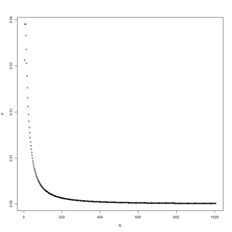
Below is just an illustration example regarding the distribution

u <- 0:500
N <- 2 * u + 5
P <- (choose(N-1, u) - choose(N-1, u + 5)) * 0.5^(N)
plot(N, P)

Prepare answered 22/1 at 0:28 Comment(2)

thank you so much for your answer! Can your code be adapted to plot the individual simulation trajectories (i.e. paths)? – Concatenate 24/1 at 2:4

@Concatenate see another answer of mine. – Prepare 24/1 at 10:45

For Situation 1

First of all, if you want to find all possible trajectories, I don't think it is efficient to capture all of them if you use "simulations" only, since the expanded space blows up when you have longer trajectories.

Appended to the question "Can your code be adapted to plot the individual simulation trajectories (i.e. paths)?" (see the comments to the answer by @ThomasIsCoding), you can enumerate all that paths using the recursion manner.

Code to Find All Trajettories

If you want to get all trajectories that departs from a source node src to the first-hit target tg with L hops, you can try the code below

f <- function(L, src, tg = 0) {
  # not available if number of hops shorter than the source-target distance
  if (L < abs(src - tg)) {
    return(list())
  }
  # there is one single path if number of hops equals to the distance
  if (L == abs(src-tg)) {
    return(list(src:tg))
  }
  if (L == 1) {
    if (src %in% (tg + c(1, -1))) {
      return(list(c(src, tg)))
    } else {
      return(NULL)
    }
  }
  # if next hop is "+1"
  if (src + 1 != tg) {
    u <- Recall(L - 1, src + 1, tg)
  } else {
    u <- NULL
  }
  # if next hop is "-1"
  if (src - 1 != tg) {
    v <- Recall(L - 1, src - 1, tg)
  } else {
    v <- NULL
  }
  # if u or v is not NULL, expand the paths with the source node
  ps <- c(u, v)
  if (!is.null(ps)) {
    Map(c, src, c(u, v))
  } else {
    list()
  }
}

Output Examples

> f(5, 5)
[[1]]
[1] 5 4 3 2 1 0


> f(6, 5)
list()

> f(7, 5)
[[1]]
[1] 5 6 5 4 3 2 1 0

[[2]]
[1] 5 4 5 4 3 2 1 0

[[3]]
[1] 5 4 3 4 3 2 1 0

[[4]]
[1] 5 4 3 2 3 2 1 0

[[5]]
[1] 5 4 3 2 1 2 1 0


> f(8, 5)
list()

> f(9, 5)
[[1]]
 [1] 5 6 7 6 5 4 3 2 1 0

[[2]]
 [1] 5 6 5 6 5 4 3 2 1 0

[[3]]
 [1] 5 6 5 4 5 4 3 2 1 0

[[4]]
 [1] 5 6 5 4 3 4 3 2 1 0

[[5]]
 [1] 5 6 5 4 3 2 3 2 1 0

[[6]]
 [1] 5 6 5 4 3 2 1 2 1 0

[[7]]
 [1] 5 4 5 6 5 4 3 2 1 0

[[8]]
 [1] 5 4 5 4 5 4 3 2 1 0

[[9]]
 [1] 5 4 5 4 3 4 3 2 1 0

[[10]]
 [1] 5 4 5 4 3 2 3 2 1 0

[[11]]
 [1] 5 4 5 4 3 2 1 2 1 0

[[12]]
 [1] 5 4 3 4 5 4 3 2 1 0

[[13]]
 [1] 5 4 3 4 3 4 3 2 1 0

[[14]]
 [1] 5 4 3 4 3 2 3 2 1 0

[[15]]
 [1] 5 4 3 4 3 2 1 2 1 0

[[16]]
 [1] 5 4 3 2 3 4 3 2 1 0

[[17]]
 [1] 5 4 3 2 3 2 3 2 1 0

[[18]]
 [1] 5 4 3 2 3 2 1 2 1 0

[[19]]
 [1] 5 4 3 2 1 2 3 2 1 0

[[20]]
 [1] 5 4 3 2 1 2 1 2 1 0

Trajectory Visualization

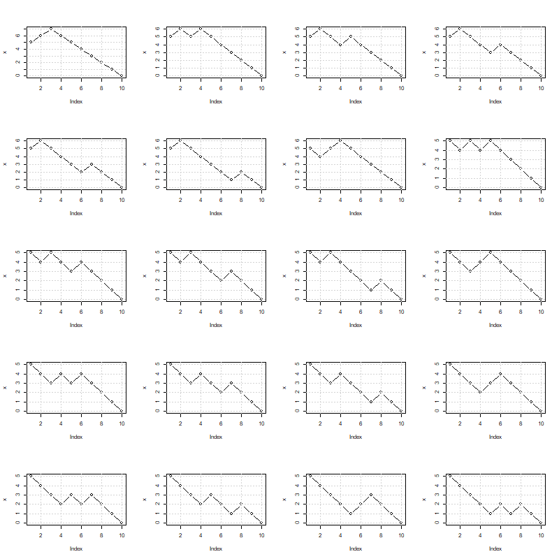
If you want to visualize all those trajectories

paths <- f(9, 5)
tryCatch(
  expr = {
    nr <- ceiling(sqrt(length(paths)))
    nc <- ceiling(length(paths) / nr)
    par(mfrow = c(nr, nc))
    invisible(lapply(paths, \(x) {
      plot(x, type = "b")
      grid()
    }))
  },
  error = function(e) {
    print("No valide paths found!")
  }
)

Prepare answered 24/1 at 10:35 Comment(1)

@Concatenate you are welcome. I added some comments in the code and hope they can help you understand the recursion easier. – Prepare 24/1 at 11:21

For Situation 2

A follow-up on top of the answer by @ThomasIsCoding, here is the code to find all possible trajectories that pass a mid-point (see Situation 2 in the question).

Code

Let L, src, mid, and tg denote the total number of hops, source node, first-hit midpoint, and first-hit target, respectively, we can try the code to generate all paths but need to the

ff <- function(L, src, mid, tg) {
  l <- abs(src - mid):(L - abs(tg - mid))
  unlist(
    lapply(
      l,
      \(k) {
        p1 <- f(k, src, mid)
        p2 <- f(L - k, mid, tg)
        if (min(length(p1), length(p2)) > 0) {
          unlist(
            lapply(p1, \(x) Map(\(a, b) c(head(a, -1), b), list(x), p2)),
            recursive = FALSE
          )
        }
      }
    ),
    recursive = FALSE
  )
}

Output Example

L <- 19
src <- 5
mid <- 10
tg <- 0
paths <- ff(L, src, mid, tg)

gives

> paths
[[1]]
 [1]  5  6  7  8  9 10 11 12 11 10  9  8  7  6  5  4  3  2  1  0

[[2]]
 [1]  5  6  7  8  9 10 11 10 11 10  9  8  7  6  5  4  3  2  1  0

[[3]]
 [1]  5  6  7  8  9 10 11 10  9 10  9  8  7  6  5  4  3  2  1  0

[[4]]
 [1]  5  6  7  8  9 10 11 10  9  8  9  8  7  6  5  4  3  2  1  0

[[5]]
 [1]  5  6  7  8  9 10 11 10  9  8  7  8  7  6  5  4  3  2  1  0

[[6]]
 [1]  5  6  7  8  9 10 11 10  9  8  7  6  7  6  5  4  3  2  1  0

[[7]]
 [1]  5  6  7  8  9 10 11 10  9  8  7  6  5  6  5  4  3  2  1  0

[[8]]
 [1]  5  6  7  8  9 10 11 10  9  8  7  6  5  4  5  4  3  2  1  0

[[9]]
 [1]  5  6  7  8  9 10 11 10  9  8  7  6  5  4  3  4  3  2  1  0

[[10]]
 [1]  5  6  7  8  9 10 11 10  9  8  7  6  5  4  3  2  3  2  1  0

[[11]]
 [1]  5  6  7  8  9 10 11 10  9  8  7  6  5  4  3  2  1  2  1  0

[[12]]
 [1]  5  6  7  8  9 10  9 10 11 10  9  8  7  6  5  4  3  2  1  0

[[13]]
 [1]  5  6  7  8  9 10  9 10  9 10  9  8  7  6  5  4  3  2  1  0

[[14]]
 [1]  5  6  7  8  9 10  9 10  9  8  9  8  7  6  5  4  3  2  1  0

[[15]]
 [1]  5  6  7  8  9 10  9 10  9  8  7  8  7  6  5  4  3  2  1  0

[[16]]
 [1]  5  6  7  8  9 10  9 10  9  8  7  6  7  6  5  4  3  2  1  0

[[17]]
 [1]  5  6  7  8  9 10  9 10  9  8  7  6  5  6  5  4  3  2  1  0

[[18]]
 [1]  5  6  7  8  9 10  9 10  9  8  7  6  5  4  5  4  3  2  1  0

[[19]]
 [1]  5  6  7  8  9 10  9 10  9  8  7  6  5  4  3  4  3  2  1  0

[[20]]
 [1]  5  6  7  8  9 10  9 10  9  8  7  6  5  4  3  2  3  2  1  0

[[21]]
 [1]  5  6  7  8  9 10  9 10  9  8  7  6  5  4  3  2  1  2  1  0

[[22]]
 [1]  5  6  7  8  9 10  9  8  9 10  9  8  7  6  5  4  3  2  1  0

[[23]]
 [1]  5  6  7  8  9 10  9  8  9  8  9  8  7  6  5  4  3  2  1  0

[[24]]
 [1]  5  6  7  8  9 10  9  8  9  8  7  8  7  6  5  4  3  2  1  0

[[25]]
 [1]  5  6  7  8  9 10  9  8  9  8  7  6  7  6  5  4  3  2  1  0

[[26]]
 [1]  5  6  7  8  9 10  9  8  9  8  7  6  5  6  5  4  3  2  1  0

[[27]]
 [1]  5  6  7  8  9 10  9  8  9  8  7  6  5  4  5  4  3  2  1  0

[[28]]
 [1]  5  6  7  8  9 10  9  8  9  8  7  6  5  4  3  4  3  2  1  0

[[29]]
 [1]  5  6  7  8  9 10  9  8  9  8  7  6  5  4  3  2  3  2  1  0

[[30]]
 [1]  5  6  7  8  9 10  9  8  9  8  7  6  5  4  3  2  1  2  1  0

[[31]]
 [1]  5  6  7  8  9 10  9  8  7  8  9  8  7  6  5  4  3  2  1  0

[[32]]
 [1]  5  6  7  8  9 10  9  8  7  8  7  8  7  6  5  4  3  2  1  0

[[33]]
 [1]  5  6  7  8  9 10  9  8  7  8  7  6  7  6  5  4  3  2  1  0

[[34]]
 [1]  5  6  7  8  9 10  9  8  7  8  7  6  5  6  5  4  3  2  1  0

[[35]]
 [1]  5  6  7  8  9 10  9  8  7  8  7  6  5  4  5  4  3  2  1  0

[[36]]
 [1]  5  6  7  8  9 10  9  8  7  8  7  6  5  4  3  4  3  2  1  0

[[37]]
 [1]  5  6  7  8  9 10  9  8  7  8  7  6  5  4  3  2  3  2  1  0

[[38]]
 [1]  5  6  7  8  9 10  9  8  7  8  7  6  5  4  3  2  1  2  1  0

[[39]]
 [1]  5  6  7  8  9 10  9  8  7  6  7  8  7  6  5  4  3  2  1  0

[[40]]
 [1]  5  6  7  8  9 10  9  8  7  6  7  6  7  6  5  4  3  2  1  0

[[41]]
 [1]  5  6  7  8  9 10  9  8  7  6  7  6  5  6  5  4  3  2  1  0

[[42]]
 [1]  5  6  7  8  9 10  9  8  7  6  7  6  5  4  5  4  3  2  1  0

[[43]]
 [1]  5  6  7  8  9 10  9  8  7  6  7  6  5  4  3  4  3  2  1  0

[[44]]
 [1]  5  6  7  8  9 10  9  8  7  6  7  6  5  4  3  2  3  2  1  0

[[45]]
 [1]  5  6  7  8  9 10  9  8  7  6  7  6  5  4  3  2  1  2  1  0

[[46]]
 [1]  5  6  7  8  9 10  9  8  7  6  5  6  7  6  5  4  3  2  1  0

[[47]]
 [1]  5  6  7  8  9 10  9  8  7  6  5  6  5  6  5  4  3  2  1  0

[[48]]
 [1]  5  6  7  8  9 10  9  8  7  6  5  6  5  4  5  4  3  2  1  0

[[49]]
 [1]  5  6  7  8  9 10  9  8  7  6  5  6  5  4  3  4  3  2  1  0

[[50]]
 [1]  5  6  7  8  9 10  9  8  7  6  5  6  5  4  3  2  3  2  1  0

[[51]]
 [1]  5  6  7  8  9 10  9  8  7  6  5  6  5  4  3  2  1  2  1  0

[[52]]
 [1]  5  6  7  8  9 10  9  8  7  6  5  4  5  6  5  4  3  2  1  0

[[53]]
 [1]  5  6  7  8  9 10  9  8  7  6  5  4  5  4  5  4  3  2  1  0

[[54]]
 [1]  5  6  7  8  9 10  9  8  7  6  5  4  5  4  3  4  3  2  1  0

[[55]]
 [1]  5  6  7  8  9 10  9  8  7  6  5  4  5  4  3  2  3  2  1  0

[[56]]
 [1]  5  6  7  8  9 10  9  8  7  6  5  4  5  4  3  2  1  2  1  0

[[57]]
 [1]  5  6  7  8  9 10  9  8  7  6  5  4  3  4  5  4  3  2  1  0

[[58]]
 [1]  5  6  7  8  9 10  9  8  7  6  5  4  3  4  3  4  3  2  1  0

[[59]]
 [1]  5  6  7  8  9 10  9  8  7  6  5  4  3  4  3  2  3  2  1  0

[[60]]
 [1]  5  6  7  8  9 10  9  8  7  6  5  4  3  4  3  2  1  2  1  0

[[61]]
 [1]  5  6  7  8  9 10  9  8  7  6  5  4  3  2  3  4  3  2  1  0

[[62]]
 [1]  5  6  7  8  9 10  9  8  7  6  5  4  3  2  3  2  3  2  1  0

[[63]]
 [1]  5  6  7  8  9 10  9  8  7  6  5  4  3  2  3  2  1  2  1  0

[[64]]
 [1]  5  6  7  8  9 10  9  8  7  6  5  4  3  2  1  2  3  2  1  0

[[65]]
 [1]  5  6  7  8  9 10  9  8  7  6  5  4  3  2  1  2  1  2  1  0

[[66]]
 [1]  5  6  7  8  9  8  9 10 11 10  9  8  7  6  5  4  3  2  1  0

[[67]]
 [1]  5  6  7  8  9  8  9 10  9 10  9  8  7  6  5  4  3  2  1  0

[[68]]
 [1]  5  6  7  8  9  8  9 10  9  8  9  8  7  6  5  4  3  2  1  0

[[69]]
 [1]  5  6  7  8  9  8  9 10  9  8  7  8  7  6  5  4  3  2  1  0

[[70]]
 [1]  5  6  7  8  9  8  9 10  9  8  7  6  7  6  5  4  3  2  1  0

[[71]]
 [1]  5  6  7  8  9  8  9 10  9  8  7  6  5  6  5  4  3  2  1  0

[[72]]
 [1]  5  6  7  8  9  8  9 10  9  8  7  6  5  4  5  4  3  2  1  0

[[73]]
 [1]  5  6  7  8  9  8  9 10  9  8  7  6  5  4  3  4  3  2  1  0

[[74]]
 [1]  5  6  7  8  9  8  9 10  9  8  7  6  5  4  3  2  3  2  1  0

[[75]]
 [1]  5  6  7  8  9  8  9 10  9  8  7  6  5  4  3  2  1  2  1  0

[[76]]
 [1]  5  6  7  8  7  8  9 10 11 10  9  8  7  6  5  4  3  2  1  0

[[77]]
 [1]  5  6  7  8  7  8  9 10  9 10  9  8  7  6  5  4  3  2  1  0

[[78]]
 [1]  5  6  7  8  7  8  9 10  9  8  9  8  7  6  5  4  3  2  1  0

[[79]]
 [1]  5  6  7  8  7  8  9 10  9  8  7  8  7  6  5  4  3  2  1  0

[[80]]
 [1]  5  6  7  8  7  8  9 10  9  8  7  6  7  6  5  4  3  2  1  0

[[81]]
 [1]  5  6  7  8  7  8  9 10  9  8  7  6  5  6  5  4  3  2  1  0

[[82]]
 [1]  5  6  7  8  7  8  9 10  9  8  7  6  5  4  5  4  3  2  1  0

[[83]]
 [1]  5  6  7  8  7  8  9 10  9  8  7  6  5  4  3  4  3  2  1  0

[[84]]
 [1]  5  6  7  8  7  8  9 10  9  8  7  6  5  4  3  2  3  2  1  0

[[85]]
 [1]  5  6  7  8  7  8  9 10  9  8  7  6  5  4  3  2  1  2  1  0

[[86]]
 [1]  5  6  7  6  7  8  9 10 11 10  9  8  7  6  5  4  3  2  1  0

[[87]]
 [1]  5  6  7  6  7  8  9 10  9 10  9  8  7  6  5  4  3  2  1  0

[[88]]
 [1]  5  6  7  6  7  8  9 10  9  8  9  8  7  6  5  4  3  2  1  0

[[89]]
 [1]  5  6  7  6  7  8  9 10  9  8  7  8  7  6  5  4  3  2  1  0

[[90]]
 [1]  5  6  7  6  7  8  9 10  9  8  7  6  7  6  5  4  3  2  1  0

[[91]]
 [1]  5  6  7  6  7  8  9 10  9  8  7  6  5  6  5  4  3  2  1  0

[[92]]
 [1]  5  6  7  6  7  8  9 10  9  8  7  6  5  4  5  4  3  2  1  0

[[93]]
 [1]  5  6  7  6  7  8  9 10  9  8  7  6  5  4  3  4  3  2  1  0

[[94]]
 [1]  5  6  7  6  7  8  9 10  9  8  7  6  5  4  3  2  3  2  1  0

[[95]]
 [1]  5  6  7  6  7  8  9 10  9  8  7  6  5  4  3  2  1  2  1  0

[[96]]
 [1]  5  6  5  6  7  8  9 10 11 10  9  8  7  6  5  4  3  2  1  0

[[97]]
 [1]  5  6  5  6  7  8  9 10  9 10  9  8  7  6  5  4  3  2  1  0

[[98]]
 [1]  5  6  5  6  7  8  9 10  9  8  9  8  7  6  5  4  3  2  1  0

[[99]]
 [1]  5  6  5  6  7  8  9 10  9  8  7  8  7  6  5  4  3  2  1  0

[[100]]
 [1]  5  6  5  6  7  8  9 10  9  8  7  6  7  6  5  4  3  2  1  0

[[101]]
 [1]  5  6  5  6  7  8  9 10  9  8  7  6  5  6  5  4  3  2  1  0

[[102]]
 [1]  5  6  5  6  7  8  9 10  9  8  7  6  5  4  5  4  3  2  1  0

[[103]]
 [1]  5  6  5  6  7  8  9 10  9  8  7  6  5  4  3  4  3  2  1  0

[[104]]
 [1]  5  6  5  6  7  8  9 10  9  8  7  6  5  4  3  2  3  2  1  0

[[105]]
 [1]  5  6  5  6  7  8  9 10  9  8  7  6  5  4  3  2  1  2  1  0

[[106]]
 [1]  5  4  5  6  7  8  9 10 11 10  9  8  7  6  5  4  3  2  1  0

[[107]]
 [1]  5  4  5  6  7  8  9 10  9 10  9  8  7  6  5  4  3  2  1  0

[[108]]
 [1]  5  4  5  6  7  8  9 10  9  8  9  8  7  6  5  4  3  2  1  0

[[109]]
 [1]  5  4  5  6  7  8  9 10  9  8  7  8  7  6  5  4  3  2  1  0

[[110]]
 [1]  5  4  5  6  7  8  9 10  9  8  7  6  7  6  5  4  3  2  1  0

[[111]]
 [1]  5  4  5  6  7  8  9 10  9  8  7  6  5  6  5  4  3  2  1  0

[[112]]
 [1]  5  4  5  6  7  8  9 10  9  8  7  6  5  4  5  4  3  2  1  0

[[113]]
 [1]  5  4  5  6  7  8  9 10  9  8  7  6  5  4  3  4  3  2  1  0

[[114]]
 [1]  5  4  5  6  7  8  9 10  9  8  7  6  5  4  3  2  3  2  1  0

[[115]]
 [1]  5  4  5  6  7  8  9 10  9  8  7  6  5  4  3  2  1  2  1  0

[[116]]
 [1]  5  6  7  8  9  8  9  8  9 10  9  8  7  6  5  4  3  2  1  0

[[117]]
 [1]  5  6  7  8  9  8  7  8  9 10  9  8  7  6  5  4  3  2  1  0

[[118]]
 [1]  5  6  7  8  7  8  9  8  9 10  9  8  7  6  5  4  3  2  1  0

[[119]]
 [1]  5  6  7  8  7  8  7  8  9 10  9  8  7  6  5  4  3  2  1  0

[[120]]
 [1]  5  6  7  8  7  6  7  8  9 10  9  8  7  6  5  4  3  2  1  0

[[121]]
 [1]  5  6  7  6  7  8  9  8  9 10  9  8  7  6  5  4  3  2  1  0

[[122]]
 [1]  5  6  7  6  7  8  7  8  9 10  9  8  7  6  5  4  3  2  1  0

[[123]]
 [1]  5  6  7  6  7  6  7  8  9 10  9  8  7  6  5  4  3  2  1  0

[[124]]
 [1]  5  6  7  6  5  6  7  8  9 10  9  8  7  6  5  4  3  2  1  0

[[125]]
 [1]  5  6  5  6  7  8  9  8  9 10  9  8  7  6  5  4  3  2  1  0

[[126]]
 [1]  5  6  5  6  7  8  7  8  9 10  9  8  7  6  5  4  3  2  1  0

[[127]]
 [1]  5  6  5  6  7  6  7  8  9 10  9  8  7  6  5  4  3  2  1  0

[[128]]
 [1]  5  6  5  6  5  6  7  8  9 10  9  8  7  6  5  4  3  2  1  0

[[129]]
 [1]  5  6  5  4  5  6  7  8  9 10  9  8  7  6  5  4  3  2  1  0

[[130]]
 [1]  5  4  5  6  7  8  9  8  9 10  9  8  7  6  5  4  3  2  1  0

[[131]]
 [1]  5  4  5  6  7  8  7  8  9 10  9  8  7  6  5  4  3  2  1  0

[[132]]
 [1]  5  4  5  6  7  6  7  8  9 10  9  8  7  6  5  4  3  2  1  0

[[133]]
 [1]  5  4  5  6  5  6  7  8  9 10  9  8  7  6  5  4  3  2  1  0

[[134]]
 [1]  5  4  5  4  5  6  7  8  9 10  9  8  7  6  5  4  3  2  1  0

[[135]]
 [1]  5  4  3  4  5  6  7  8  9 10  9  8  7  6  5  4  3  2  1  0

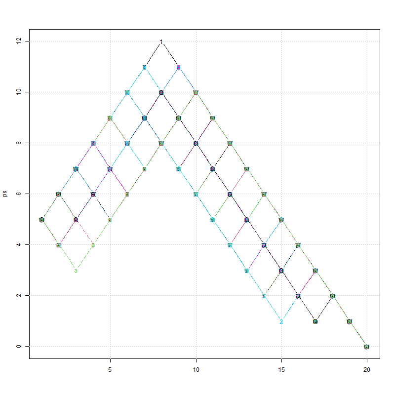
Trajectory Visualization

ps <- do.call(cbind, paths)
matplot(ps, type = "b")
grid()

shows

Prepare answered 24/1 at 14:52 Comment(0)

Hot tags

Godot Unity Godot Help Programming Godot 4.X GUI GDScript 3D 2D Physics CSharp Godot 3.X VR XR Projects C++

Function

Plotting Results

Function

Plotting Results

For Situation 1

Code to Find All Trajettories

Output Examples

Trajectory Visualization

For Situation 2

Code

Output Example

Trajectory Visualization

Recommended topics

Hot tags