Ratio of polynomials approximation

Question

I am trying to fit a polynomial to my dataset, which looks like that (full dataset is at the end of the post):

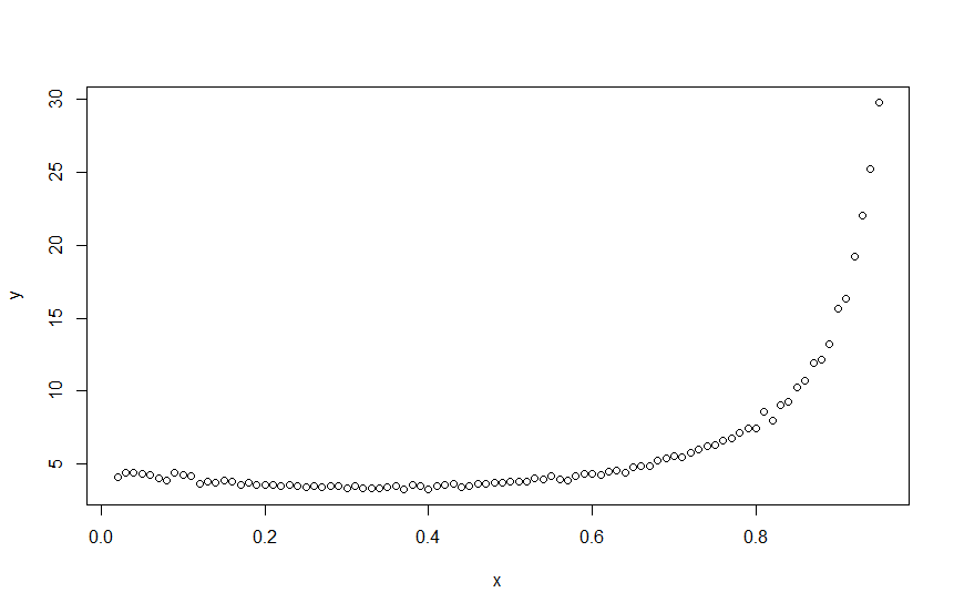
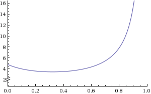
The theory predicts that the formulation of the curve is:

which looks like this (for x between 0 and 1):

When I try to make a linear model in R by doing:

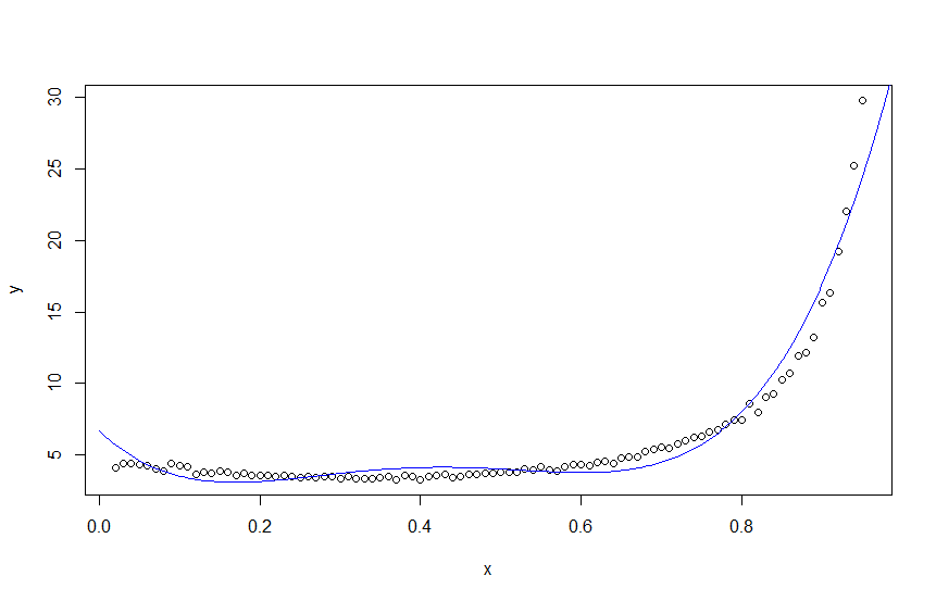
mod <- lm(y ~ poly(x, 2, raw=TRUE)/poly(x, 2))

I get the following curve:

Which is much different from what I would expect. Have you got any idea how to fit a new curve from this data so that it would be similar to the one, which theory predicts? Also, it should have only one minimum.

Full dataset:

---

Vector of x values:

x <- c(0.02, 0.03, 0.04, 0.05, 0.06, 0.07, 0.08, 0.09, 0.10, 0.11, 0.12,
 0.13, 0.14, 0.15, 0.16, 0.17, 0.18, 0.19, 0.20, 0.21, 0.22, 0.23, 0.24, 0.25,
 0.26, 0.27, 0.28, 0.29, 0.30, 0.31, 0.32, 0.33, 0.34, 0.35, 0.36, 0.37, 0.38,
 0.39, 0.40, 0.41, 0.42, 0.43, 0.44, 0.45, 0.46, 0.47, 0.48, 0.49, 0.50, 0.51,
 0.52, 0.53, 0.54, 0.55, 0.56, 0.57, 0.58, 0.59, 0.60, 0.61, 0.62, 0.63, 0.64,
 0.65, 0.66, 0.67, 0.68, 0.69, 0.70, 0.71, 0.72, 0.73, 0.74, 0.75, 0.76, 0.77,
 0.78, 0.79, 0.80, 0.81, 0.82, 0.83, 0.84, 0.85, 0.86, 0.87, 0.88, 0.89, 0.90,
 0.91, 0.92, 0.93, 0.94, 0.95)

Vector of y values:

y <- c(4.104,  4.444,  4.432,  4.334,  4.285,  4.058,  3.901,  4.382,
  4.258,  4.158,  3.688,  3.826,  3.724,  3.867,  3.811,  3.550,  3.736, 3.591,
  3.566,  3.566,  3.518,  3.581,  3.505,  3.454,  3.529,  3.444,  3.501,  3.493,
  3.362,  3.504,  3.365,  3.348,  3.371,  3.389,  3.506,  3.310,  3.578,  3.497,
  3.302,  3.530,  3.593,  3.630,  3.420,  3.467,  3.656,  3.644,  3.715,  3.698,
  3.807,  3.836,  3.826,  4.017,  3.942,  4.208,  3.959,  3.856,  4.157,  4.312,
  4.349,  4.286,  4.483,  4.599,  4.395,  4.811,  4.887,  4.885,  5.286,  5.422,
  5.527,  5.467,  5.749,  5.980,  6.242,  6.314,  6.587,  6.790,  7.183,  7.450,
  7.487,  8.566,  7.946,  9.078,  9.308, 10.267, 10.738, 11.922, 12.178, 13.243,
  15.627, 16.308, 19.246, 22.022, 25.223, 29.752)

Pamulapan

The ratio of two polynomials will not be estimated by a linear model. You need to use nonlinear methods. – Nymphet

Answer 1

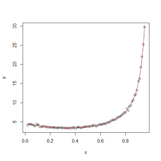
Use nls to fit a nonlinear model. Note that the model formula is not uniquely defined as displayed in the question since if we multiply all the coefficients by any number the result will still give the same predictions. To avoid this we need to fix one coefficient. A first try used the coefficients shown in the question as starting values (except fixing one) but that failed so dropping C was tried and the resulting coefficients fed into a second fit with C = 1.

 st <- list(a = 43, b = -14, c = 25, B = 18)
 fm <- nls(y ~ (a + b * x + c * x^2) / (9 + B * x), start = st)
 fm2 <- nls(y ~ (a + b * x + c * x^2) / (9 + B * x + C * x^2), start = c(coef(fm), C = 1))

 plot(y ~ x)
 lines(fitted(fm2) ~ x, col = "red")

(continued after chart)

Note: Here is an example of using nls2 to get starting values with random search. We assume that the coefficients each lie between -50 and 50.

library(nls2)

set.seed(123) # for reproducibility
v <- c(a = 50, b = 50, c = 50, B = 50, C = 50)
st0 <- as.data.frame(rbind(-v, v))
fm0 <- nls2(y ~ (a + b * x + c * x^2) / (9 + B * x + C * x^2), start = st0,
   alg = "random", control = list(maxiter = 1000))

fm3 <- nls(y ~ (a + b * x + c * x^2) / (9 + B * x + C * x^2), st = coef(fm0))

Perspiration

Thank you very much! However, it produces and error "Error in coef(fm) : object 'fm' not found". How could we overcome it? – Pamulapan

You would need an earlier fm object to exist in the workspace for that code to succeed (which Gabor had alluded to). Instead you get an estimate with nls(y ~ (a + b * x + c * x^2) / (9 + B * x + C * x^2), start = st). It's kind of interesting to see how unstable the individual parameters are. – Nymphet

Have revised solution. – Perspiration

What if we have a different grap and have not much idea about starting value? Is there any general method? – Pamulapan

If you have an idea of the range that the coefficients lie in then you can use a brute force or random search using the nls2 package and then use the best coefficients found with that as your nls starting values. See the examples that come with nls2. – Perspiration

Answer 2

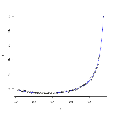
Since you already have a theoretic prediction, you don't seem in need of a new model, and it's really only a plotting task:

 png(); plot(y~x)
 lines(x,mod,col="blue")
 dev.off()

You cannot expect lm to produce a good approximation to a non-linear problem. The denominator involving x in that theoretic expression makes this inherently nonlinear.

Nymphet

In this case it is a plotting task, but I would just like to know how to do it in general, for example assuming we do not know the theoretic formula. – Pamulapan

The last sentence in this answer is decisive. This is not a linear problem, and because of the denominator the formula cannot be approximated properly by a second-order polynomial. – Thissa

Thank you very much for your help. – Pamulapan