What is the difference between linear regression and logistic regression? [closed]

Question

When we have to predict the value of a categorical (or discrete) outcome we use logistic regression. I believe we use linear regression to also predict the value of an outcome given the input values.

Then, what is the difference between the two methodologies?

Graven

I’m voting to close this question because Machine learning (ML) theory questions are off-topic on Stack Overflow - gift-wrap candidate for Cross-Validated – Hautemarne

Answer 1

• Linear regression output as probabilities

  It's tempting to use the linear regression output as probabilities but it's a mistake because the output can be negative, and greater than 1 whereas probability can not. As regression might actually produce probabilities that could be less than 0, or even bigger than 1, logistic regression was introduced.

  Source: http://gerardnico.com/wiki/data_mining/simple_logistic_regression

• Outcome

  In linear regression, the outcome (dependent variable) is continuous. It can have any one of an infinite number of possible values.

  In logistic regression, the outcome (dependent variable) has only a limited number of possible values.

• The dependent variable

  Logistic regression is used when the response variable is categorical in nature. For instance, yes/no, true/false, red/green/blue, 1st/2nd/3rd/4th, etc.

  Linear regression is used when your response variable is continuous. For instance, weight, height, number of hours, etc.

• Equation

  Linear regression gives an equation which is of the form Y = mX + C, means equation with degree 1.

  However, logistic regression gives an equation which is of the form Y = e^X + e^-X

• Coefficient interpretation

  In linear regression, the coefficient interpretation of independent variables are quite straightforward (i.e. holding all other variables constant, with a unit increase in this variable, the dependent variable is expected to increase/decrease by xxx).

  However, in logistic regression, depends on the family (binomial, Poisson, etc.) and link (log, logit, inverse-log, etc.) you use, the interpretation is different.

• Error minimization technique

  Linear regression uses ordinary least squares method to minimise the errors and arrive at a best possible fit, while logistic regression uses maximum likelihood method to arrive at the solution.

  Linear regression is usually solved by minimizing the least squares error of the model to the data, therefore large errors are penalized quadratically.

  Logistic regression is just the opposite. Using the logistic loss function causes large errors to be penalized to an asymptotically constant.

  Consider linear regression on categorical {0, 1} outcomes to see why this is a problem. If your model predicts the outcome is 38, when the truth is 1, you've lost nothing. Linear regression would try to reduce that 38, logistic wouldn't (as much)².

Obaza

Is there a difference between Y = e^X/1 + e^-X and Y = e^X + e^-X ? – Puffery

e^X/1 ? anything divide by 1 is the same. so there is no difference. I am sure you were meaning to ask something else. – Frankfrankalmoign

I know this is an old thread but given your statement "Logistic regression is used when the response variable is categorical in nature. For instance, yes/no, true/false, red/green/blue, 1st/2nd/3rd/4th, etc. "; what's the difference between this and classification then? – Stulin

@Stulin Logistic regression is indeed used for classification. Check this out, you might find it useful as I have – Trinitrocresol

@kingJulian: Logistic regression is a classification technique and classification stands for several algorithms that try to predict few outcomes. – Provencher

to put it simply, the difference is linear regression predicts a continuous value whereas logistic predicts a discrete value. For example, predicting customer revenue based on inputs of customer transactions and some sort of expense would be linear ($100,000.75) and predicting whether a business will lose a customer (yes/no) based on inputs of transaction count or maybe prices would be logistic. – Ditter

No, linear regression and logistic regression both predict a continuous value. Linear regression predicts a continuous value in (-inf, inf) and logistic regression predicts a continuous probability in [0, 1]. We use logistic regression for classification through the use of a threshold, e.g. if the probability given by the logistic regression is >= 0.6 then we will classify it as 1, and 0 otherwise. – Psychomancy

Answer 2

In linear regression, the outcome (dependent variable) is continuous. It can have any one of an infinite number of possible values. In logistic regression, the outcome (dependent variable) has only a limited number of possible values.

For instance, if X contains the area in square feet of houses, and Y contains the corresponding sale price of those houses, you could use linear regression to predict selling price as a function of house size. While the possible selling price may not actually be any, there are so many possible values that a linear regression model would be chosen.

If, instead, you wanted to predict, based on size, whether a house would sell for more than $200K, you would use logistic regression. The possible outputs are either Yes, the house will sell for more than $200K, or No, the house will not.

Cornelius

In andrews logistic regression example of cancer, I can draw a horizontal line y=.5, (which obviously passes through y=.5 ), ten if any point is above this line y=.5 => +ve , else -ve. So then why do I need a logistic regression. Im just trying to understand the best case explanation to use logistic regression ? – Shoffner

@vinita: here or here is a simple example for not using linear regression and then thresh holding, for classification problems. – Lauber

logistic regression is the better classifier on categorical data than linear regression. It uses a cross-entropy error function instead of least squares. Therfore it isn't that sensitify to outliers and also doesn't punish "too correct" data points like least-squares does. – Berni

Answer 3

Just to add on the previous answers.

Linear regression

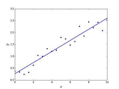
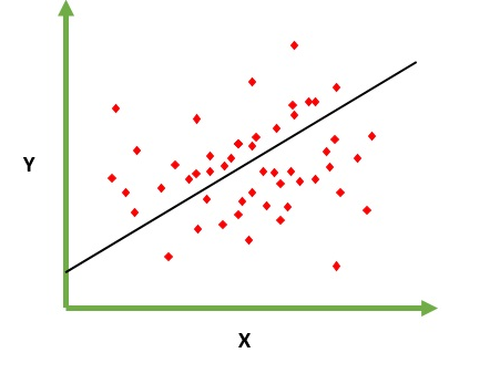
Is meant to resolve the problem of predicting/estimating the output value for a given element X (say f(x)). The result of the prediction is a continuous function where the values may be positive or negative. In this case you normally have an input dataset with lots of examples and the output value for each one of them. The goal is to be able to fit a model to this data set so you are able to predict that output for new different/never seen elements. Following is the classical example of fitting a line to set of points, but in general linear regression could be used to fit more complex models (using higher polynomial degrees):

Resolving the problem

Linear regression can be solved in two different ways:

1. Normal equation (direct way to solve the problem)
2. Gradient descent (Iterative approach)

Logistic regression

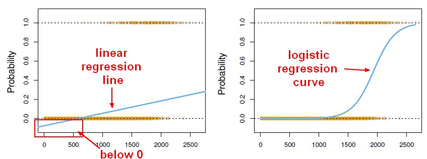
Is meant to resolve classification problems where given an element you have to classify the same in N categories. Typical examples are, for example, given a mail to classify it as spam or not, or given a vehicle find to which category it belongs (car, truck, van, etc ..). That's basically the output is a finite set of discrete values.

Resolving the problem

Logistic regression problems could be resolved only by using Gradient descent. The formulation in general is very similar to linear regression the only difference is the usage of different hypothesis function. In linear regression the hypothesis has the form:

h(x) = theta_0 + theta_1*x_1 + theta_2*x_2 .. 

where theta is the model we are trying to fit and [1, x_1, x_2, ..] is the input vector. In logistic regression the hypothesis function is different:

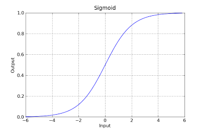
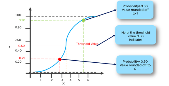
g(x) = 1 / (1 + e^-x)

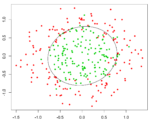
This function has a nice property, basically it maps any value to the range [0,1] which is appropiate to handle propababilities during the classificatin. For example in case of a binary classification g(X) could be interpreted as the probability to belong to the positive class. In this case normally you have different classes that are separated with a decision boundary which basically a curve that decides the separation between the different classes. Following is an example of dataset separated in two classes.

1. You can also use the below code to generate the linear regression curve q_df = details_df # q_df = pd.get_dummies(q_df)

   q_df = pd.get_dummies(q_df, columns=[
       "1",
       "2",
       "3",
       "4",
       "5",
       "6",
       "7",
       "8",
       "9"
   ])
   
   q_1_df = q_df["1"]
   q_df = q_df.drop(["2", "3", "4", "5"], axis=1)
   
   (import statsmodels.api as sm)
   
   x = sm.add_constant(q_df)
   train_x, test_x, train_y, test_y =    sklearn.model_selection.train_test_split(
   x, q3_rechange_delay_df, test_size=0.2, random_state=123 )
   

   lmod = sm.OLS(train_y, train_x).fit() lmod.summary()

   lmod.predict()[:10]

   lmod.get_prediction().summary_frame()[:10]

   sm.qqplot(lmod.resid,line="q") plt.title("Q-Q plot of Standardized Residuals") plt.show()

Assoil

Answer 4

The basic difference :

Linear regression is basically a regression model which means its will give a non discreet/continuous output of a function. So this approach gives the value. For example : given x what is f(x)

For example given a training set of different factors and the price of a property after training we can provide the required factors to determine what will be the property price.

Logistic regression is basically a binary classification algorithm which means that here there will be discreet valued output for the function . For example : for a given x if f(x)>threshold classify it to be 1 else classify it to be 0.

For example given a set of brain tumour size as training data we can use the size as input to determine whether its a benine or malignant tumour. Therefore here the output is discreet either 0 or 1.

*here the function is basically the hypothesis function

Poet

Answer 5

They are both quite similar in solving for the solution, but as others have said, one (Logistic Regression) is for predicting a category "fit" (Y/N or 1/0), and the other (Linear Regression) is for predicting a value.

So if you want to predict if you have cancer Y/N (or a probability) - use logistic. If you want to know how many years you will live to - use Linear Regression !

Bodhisattva

Answer 6

Simply put, linear regression is a regression algorithm, which outpus a possible continous and infinite value; logistic regression is considered as a binary classifier algorithm, which outputs the 'probability' of the input belonging to a label (0 or 1).

Vizard

Thank goodness I read your note about probability. Was about to write off logistic as a binary classifier. – Glorianna

Answer 7

Regression means continuous variable, Linear means there is linear relation between y and x. Ex= You are trying to predict salary from no of years of experience. So here salary is independent variable(y) and yrs of experience is dependent variable(x). y=b0+ b1*x1 We are trying to find optimum value of constant b0 and b1 which will give us best fitting line for your observation data. It is a equation of line which gives continuous value from x=0 to very large value. This line is called Linear regression model.

Logistic regression is type of classification technique. Dnt be misled by term regression. Here we predict whether y=0 or 1.

Here we first need to find p(y=1) (wprobability of y=1) given x from formuale below.

Probaibility p is related to y by below formuale

Ex=we can make classification of tumour having more than 50% chance of having cancer as 1 and tumour having less than 50% chance of having cancer as 0.

Here red point will be predicted as 0 whereas green point will be predicted as 1.

Vue

Answer 8

Cannot agree more with the above comments. Above that, there are some more differences like

In Linear Regression, residuals are assumed to be normally distributed. In Logistic Regression, residuals need to be independent but not normally distributed.

Linear Regression assumes that a constant change in the value of the explanatory variable results in constant change in the response variable. This assumption does not hold if the value of the response variable represents a probability (in Logistic Regression)

GLM(Generalized linear models) does not assume a linear relationship between dependent and independent variables. However, it assumes a linear relationship between link function and independent variables in logit model.

Lyonnaise

Answer 9

In short: Linear Regression gives continuous output. i.e. any value between a range of values. Logistic Regression gives discrete output. i.e. Yes/No, 0/1 kind of outputs.

Bradeord

Answer 10

To put it simply, if in linear regression model more test cases arrive which are far away from the threshold(say =0.5)for a prediction of y=1 and y=0. Then in that case the hypothesis will change and become worse.Therefore linear regression model is not used for classification problem.

Another Problem is that if the classification is y=0 and y=1, h(x) can be > 1 or < 0.So we use Logistic regression were 0<=h(x)<=1.

Ferocious

Answer 11

| Basis                                                           | Linear                                                                         | Logistic                                                                                                            |
|-----------------------------------------------------------------|--------------------------------------------------------------------------------|---------------------------------------------------------------------------------------------------------------------|
| Basic                                                           | The data is modelled using a straight line.                                    | The probability of some obtained event is represented as a linear function of a combination of predictor variables. |
| Linear relationship between dependent and independent variables | Is required                                                                    | Not required                                                                                                        |
| The independent variable                                        | Could be correlated with each other. (Specially in multiple linear regression) | Should not be correlated with each other (no multicollinearity exist).                                              |

Robertaroberto

Answer 12

Logistic Regression is used in predicting categorical outputs like Yes/No, Low/Medium/High etc. You have basically 2 types of logistic regression Binary Logistic Regression (Yes/No, Approved/Disapproved) or Multi-class Logistic regression (Low/Medium/High, digits from 0-9 etc)

On the other hand, linear regression is if your dependent variable (y) is continuous. y = mx + c is a simple linear regression equation (m = slope and c is the y-intercept). Multilinear regression has more than 1 independent variable (x1,x2,x3 ... etc)

Reconvert

Answer 13

In linear regression the outcome is continuous whereas in logistic regression, the outcome has only a limited number of possible values(discrete).

example: In a scenario,the given value of x is size of a plot in square feet then predicting y ie rate of the plot comes under linear regression.

If, instead, you wanted to predict, based on size, whether the plot would sell for more than 300000 Rs, you would use logistic regression. The possible outputs are either Yes, the plot will sell for more than 300000 Rs, or No.

Larcener

Answer 14

In case of Linear Regression the outcome is continuous while in case of Logistic Regression outcome is discrete (not continuous)

To perform Linear regression we require a linear relationship between the dependent and independent variables. But to perform Logistic regression we do not require a linear relationship between the dependent and independent variables.

Linear Regression is all about fitting a straight line in the data while Logistic Regression is about fitting a curve to the data.

Linear Regression is a regression algorithm for Machine Learning while Logistic Regression is a classification Algorithm for machine learning.

Linear regression assumes gaussian (or normal) distribution of dependent variable. Logistic regression assumes binomial distribution of dependent variable.

Homerhomere

Answer 15

The basic difference between Linear Regression and Logistic Regression is : Linear Regression is used to predict a continuous or numerical value but when we are looking for predicting a value that is categorical Logistic Regression come into picture.

Logistic Regression is used for binary classification.

Psf