What are fitness sharing and niche count in evolutionary computation?

Question

What are "fitness sharing" and "niche count" in the context of evolutionary computation?

Stumper

Answer 1

Evolutionary algorithms (EAs) tend to converge to a single solution as the diversity of the population diminishes [1]. This behavior is known as genetic drift. Any technique that maintains diversity in the population based on the distance between the population members is called a Niching technique.

Fitness sharing is a type of Niching, where the fitness of each individual is scaled based on its proximity to others. This means that good solutions in densely populated regions are given a lower fitness value than comparably good solutions in sparsely populated regions. In effect, the algorithm's selection technique places less emphasis on these high-quality, high-density solutions. The distance can be calculated based on the values in either decision space (genotype), solution space (phenotype), or both (as in Goldberg and Richardsen [2]). Distance in genotype is usually defined using the Hamming distance whereas distance in phenotype is usually defined using Euclidean distance.

A simple fitness sharing method is given by the following Java method:

    /** 
    * Computes the shared fitness value for a solution
    * @param index the index of the solution for which a shared fitness value will be computed
    * @param minDist any solution closer than minDist will share fitness with the current solution
    * @param shareParam a parameter that defines how much influence sharing has. Higher = more sharing.
    * @param population the array of solutions. Each solution has a genotype and associated fitness value.
    */
    public double computeSharedFitnessValue(int index, double minDist, double shareParam, Solution[] population){
      
      double denominator = 1;
      
      for(int j = 0; j < population.length; j++){
      
         final double dist = hamming_dist(population[index],population[j]);
      
         if (dist < minDist){
            denominator += (1-(dist/shareParam))
         }
      }
      
      return population[index].getFitnessValue()/denominator;
    }

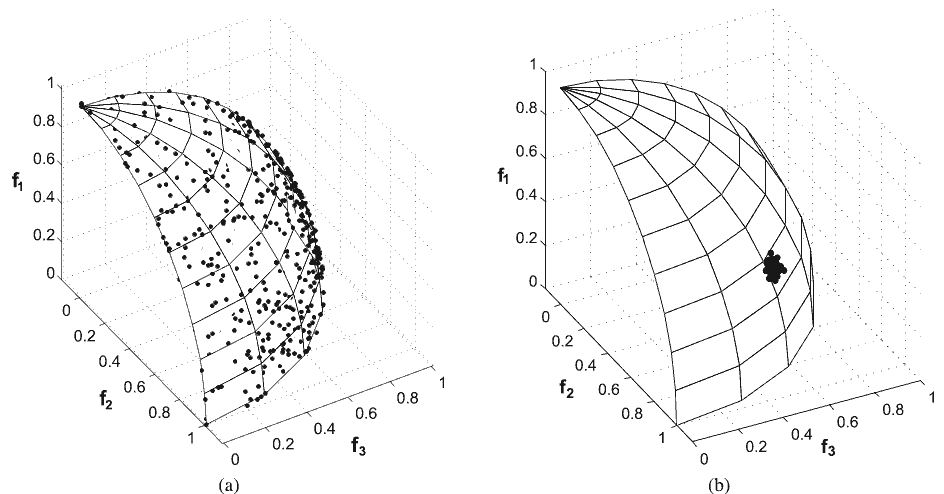
Motivational Example: The following figure perfectly illustrates why fitness sharing is so important in multi-objective problems. In Figure A (left), diversity was maintained throughout execution. As a result, the solutions span a considerable portion of the true Pareto front (shown here as wire frame). In Figure B (right), the population only converged to a small area of the Pareto front. In many situations, even if the solutions in Figure B were of higher quality, a decision maker would prefer the diversity of options provided in Figure A to the (nominal) improvement in quality of Figure B.

Additional Resources:

• [1] Genetic algorithms with sharing for multimodal function optimization
• [2] Genetic Algorithms for Multi-Objective Optimization: Formulation Discussion and Generalization

Boomkin

Great answer. Could you expand on the difference between explicit and implicit fitness sharing? – Soileau

@Soileau Implicit fitness sharing differs from the explicit form in that no explicit distance metric is required. – Boomkin