How to convert a spline fit into a piecewise function?

Question

Let's say I have

import numpy as np
from scipy.interpolate import UnivariateSpline

# "true" data; I don't know this function
x = np.linspace(0, 100, 1000)
d = np.sin(x * 0.5) + 2 + np.cos(x * 0.1)

# sample data; that's what I actually measured
x_sample = x[::20]
d_sample = d[::20]

# fit spline
s = UnivariateSpline(x_sample, d_sample, k=3, s=0.005)

plt.plot(x, d)
plt.plot(x_sample, d_sample, 'o')
plt.plot(x, s(x))
plt.show()

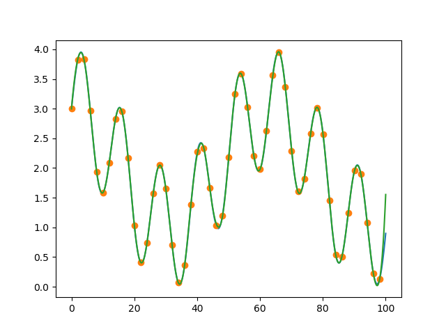
I get

What I would now like to have are functions between all the orange dots, so something like

knots = s.get_knots()
f0 = <some expression> for knots[0] <= x < knots[1]
f1 = <some expression> for knots[1] <= x < knots[2]
...

Thereby, fi should be chosen in a way that it reproduces the shape of the spline fit.

I found the post here, but the spline produced there seems incorrect for the example above and it's also not exactly what I need as it does not return expressions.

How could I turn the spline into a piecewise function? Is there a (straightforward) way to express each interval e.g. as a polynomial?

Barytone

I haven't figured this out either, but my understanding is the difficulty is converting the coefficients of the B-spline basis to coefficients of the standard power basis you want, and it's not as easy as PPoly.from_spline. Once you have the coeffs, it's a simple application of, for example, np.polyeval and np.piecewise. Have a look at this discussion on the trickiness of conversion. – Upward

@stevemo: Could you elaborate on the PPoly.from_spline part? I do not have to use UnivariateSpline, but any spline is fine that gives me fi I could then indeed feed into piecewise. – Barytone

I ended up figuring it out and gave a full answer ... can edit a bit if needed. – Upward

@stevemo: Great, thanks! Don't have time to go through it today anymore, but will do so tomorrow and then get back to you; so don't be surprised if I am silent for a while... :) – Barytone

Answer 1

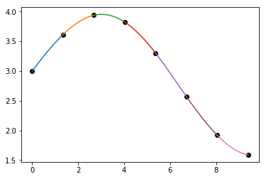
The short answer is, if you're interested in coefficients of a polynomial in standard power basis, you'd be better off using CubicSpline (and see this discussion):

cu = scipy.interpolate.CubicSpline(x_sample, d_sample)

plt.plot(x_sample, y_sample, 'ko')
for i in range(len(cu.x)-1):
    xs = np.linspace(cu.x[i], cu.x[i+1], 100)
    plt.plot(xs, np.polyval(cu.c[:,i], xs - cu.x[i]))

And to answer your question, you could instead create a piecewise function from here using numpy.piecewise, the breakpoints in cu.x and the coefficients in cu.c, and either directly code the polynomial expressions yourself or use numpy.polyval. For example,

cu.c[:,0]  # coeffs for 0th segment
# array([-0.01316353, -0.02680068,  0.51629024,  3.        ])

# equivalent ways to code polynomial for this segment
f0 = lambda x: cu.c[0,0]*(x-x[0])**3 + cu.c[1,0]*(x-x[0])**2 + cu.c[2,0]*(x-x[0]) + cu.c[3,0]
f0 = lambda x: [cu.c[i,0]*(x-x[0])**(3-i) for i in range(4)]

# ... or getting values directly from x's
y0 = np.polyval(cu.c[:,0], xs - cu.x[0])

LONGER ANSWER:

There are a few points of potential confusion here:

• UnivariateSpline fits a B-spline basis, so the coefficients are not the same as a standard polynomial power basis
• In order to convert from B-spline, we can use PPoly.from_spline, but unfortunately UnivariateSpline returns a truncated list of knots and coefficients that won't play with this function. We can resolve this problem by accessing the internal data of the spline object, which is a little taboo.
• Also, the coefficient matrix c (whether from UnivariateSpline or CubicSpline) is in reverse degree order and assumes you are "centering" yourself, e.g. the coefficient at c[k,i] belongs to c[k,i]*(x-x[i])^(3-k).

Given your setup, note that if instead of using the UnivariateSpline wrapper, we directly fit with splrep and no smoothing (s=0), we can grab the tck (knots-coefficients-degree) tuple and send it to the PPoly.from_spline function and get the coefficients we want:

tck = scipy.interpolate.splrep(x_sample, d_sample, s=0)
tck
# (array([0.        , 0.        , 0.        , 0.        , 2.68456376,
#        4.02684564, 5.36912752, 6.7114094 , 9.39597315, 9.39597315,
#        9.39597315, 9.39597315]),
# array([3.        , 3.46200469, 4.05843704, 3.89649312, 3.33792889,
#        2.29435138, 1.65015175, 1.59021688, 0.        , 0.        ,
#        0.        , 0.        ]),
# 3)

p = scipy.interpolate.PPoly.from_spline(tck)
p.x.shape  # breakpoints in unexpected shape
# (12,)

p.c.shape  # polynomial coeffs in unexpected shape
# (4, 11)

Notice the weird repeated breakpoints in tck and again in p.x: this is a FITPACK thing (the algorithm running all this).

If we try to send a tck tuple from UnivariateSpline with (s.get_knots(), s.get_coeffs(), 3), we are missing those repeats, so from_spline doesn't work. Checking out the source though it appears the full vector is stored in self._data, so we can do

s = scipy.interpolate.UnivariateSpline(x_sample, d_sample, s=0)
tck = (s._data[8], s._data[9], 3)
p = scipy.interpolate.PPoly.from_spline(tck)

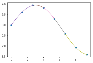
and get the same as before. To check these coefficients work:

plt.plot(x_sample, d_sample, 'o')

for i in range(len(p.x)-1):
    xs = np.linspace(p.x[i], p.x[i+1], 10)
    plt.plot(xs, np.polyval(p.c[:,i], xs - p.x[i]))

Note numpy.polyval wants reverse order for coeffs so we can pass p.c as-is.

Upward

Still did not find the time to really test it, but it looks pretty good. Just one small thing, then I accept and also award the bounty: "if you're interested in coefficients of a polynomial in standard power basis", I think that would be fine. Could you write down the analytical equation for the first three sections or so, so (just random expressions for now) f1 = x^2 + 2, f2 = x^3 + x^2 + 2,... based on the output of np.polyval? In my actual application I would need these expressions for each piece, so I cannot use numpy; if that is done, the it seems to be the perfect answer, thanks :) – Barytone

I added an example for the first segment, hopefully that helps – Upward

Answer 2

Should be able use a piecewise function as you described, something like:

import numpy as np
from scipy.interpolate import UnivariateSpline

# "true" data; I don't know this function
x = np.linspace(0, 100, 1000)
d = np.sin(x * 0.5) + 2 + np.cos(x * 0.1)

# sample data; that's what I actually measured
x_sample = x[::20]
d_sample = d[::20]

# fit spline
s = UnivariateSpline(x_sample, d_sample, k=3, s=0.005)

plt.plot(x, d)
plt.plot(x_sample, d_sample, 'o')
plt.plot(x, s(x))

knots = s.get_knots()

conditions = [x < knots[0], (x >= knots[0]) * (x < knots[1]), (x >= knots[1]) * (x < knots[10]), x >= knots[10]]
# need one function for each condition
fns = [0, lambda x :-x, lambda x: 0.01*x**2, lambda x: 0.2*x**0.5]
y = np.piecewise(x, conditions, fns)

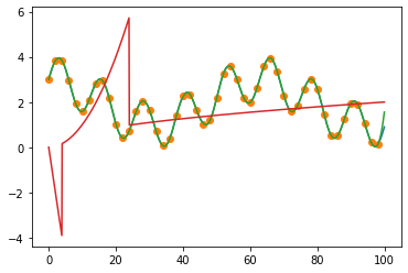
plt.plot(x, y)
plt.show()

I chose some random conditions and functions- I'm sure you could find something more suitable!

Victim

Thanks. Few questions: What is the red line? Shouldn't it have the same shape as the green and blue ones? Maybe it's not clear from my post, but I want to reproduce the exact shape of the curve, just as a piecewise function rather than using s(x). How did you construct fns, e.g. the 0.01*x**2, where does that come from? Wouldn't you also need s.get_coeffs()? – Barytone

Ah yes sorry, I thought you had might want to reconstruct the green curve but it wasn't clear. The fns I made eg. 0.01*x**2 were just to show the piecewise operation but I realise now that wasn't exactly what you were after! – Victim