matplotlib.mlab.psd(...) and scipy.signal.welch(...) both implement Welch's average periodogram method to estimate the power spectral density (PSD) of a signal. Assuming equivalent parameters are passed to each function, the returned PSD should be equivalent.
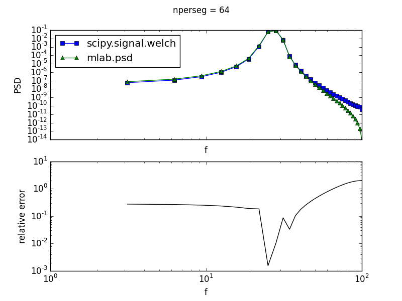
However, using a simple sinusoidal test function, there are systematic differences between the two methods when the number of points used per window (the nperseg keyword for scipy.signal.welch; the NFFT keyword for mlab.psd) is even, as shown below for the case of 64 points per window
The top plot shows the PSD computed via both methods, while the bottom plot displays their relative error (i.e. the absolute difference of the two PSDs divided by their absolute average). A larger relative error is indicative of larger disagreement between the two methods.
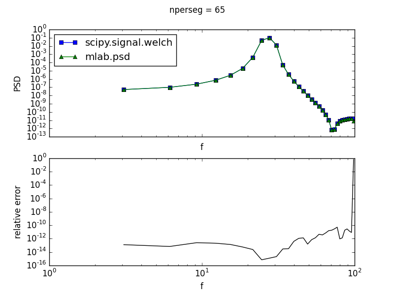
The two functions have much better agreement when the number of points used per window is odd, as shown below for the same signal but processed with 65 points per window
Adding other features to the signal (e.g. noise) somewhat diminishes this effect, but it is still present, with relative errors of ~10% between the two methods when an even number of points is used per window. (I realize the relative error at the very highest frequency for the PSDs computed with 65 points per window above is relatively large. However, this is at the signal's Nyquist frequency, and I'm not too concerned about features at such high frequencies. I'm more concerned about the large and systematic relative error across the majority of the signal's bandwidth when the number of points per window is even).
Is there a reason for this discrepancy? Is one method preferable to the other in terms of accuracy? I am using scipy version 0.16.0 and matplotlib version 1.4.3.
The code used to generate the above plots is included below. For a pure sinusoidal signal, set A_noise = 0; for a noisy signal, set A_noise to a finite value.
import numpy as np
import matplotlib.pyplot as plt
from scipy.signal import welch
from matplotlib import mlab

# Sampling information
Fs = 200.
t0 = 0
tf = 10
t = np.arange(t0, tf, 1. / Fs)

# Pure sinusoidal signal
f0 = 27.
y = np.cos(2 * np.pi * f0 * t)

# Add in some white noise
A_noise = 1e-3
y += (A_noise * np.random.randn(len(y)))

nperseg = 64    # even
# nperseg = 65  # odd

if nperseg > len(y):
    raise ValueError('nperseg > len(y); preventing unintentional zero padding')

# Compute PSD with `scipy.signal.welch`
f_welch, S_welch = welch(
    y, fs=Fs, nperseg=nperseg, noverlap=(nperseg // 2),
    detrend=None, scaling='density', window='hanning')

# Compute PSD with `matplotlib.mlab.psd`, using parameters that are
# *equivalent* to those used in `scipy.signal.welch` above
S_mlab, f_mlab = mlab.psd(
    y, Fs=Fs, NFFT=nperseg, noverlap=(nperseg // 2),
    detrend=None, scale_by_freq=True, window=mlab.window_hanning)

fig, axes = plt.subplots(2, 1, sharex=True)

# Plot PSD computed via both methods
axes[0].loglog(f_welch, S_welch, '-s')
axes[0].loglog(f_mlab, S_mlab, '-^')
axes[0].set_xlabel('f')
axes[0].set_ylabel('PSD')
axes[0].legend(['scipy.signal.welch', 'mlab.psd'], loc='upper left')

# Plot relative error
delta = np.abs(S_welch - S_mlab)
avg = 0.5 * np.abs(S_welch + S_mlab)
relative_error = delta / avg
axes[1].loglog(f_welch, relative_error, 'k')
axes[1].set_xlabel('f')
axes[1].set_ylabel('relative error')

plt.suptitle('nperseg = %i' % nperseg)
plt.show()


