How to find period of signal (autocorrelation vs fast fourier transform vs power spectral density)?

Question

Suppose one wanted to find the period of a given sinusoidal wave signal. From what I have read online, it appears that the two main approaches employ either fourier analysis or autocorrelation. I am trying to automate the process using python and my usage case is to apply this concept to similar signals that come from the time-series of positions (or speeds or accelerations) of simulated bodies orbiting a star.

For simple-examples-sake, consider x = sin(t) for 0 ≤ t ≤ 10 pi.

import numpy as np
from scipy import signal
import matplotlib.pyplot as plt

## sample data
t = np.linspace(0, 10 * np.pi, 100)
x = np.sin(t)
fig, ax = plt.subplots()
ax.plot(t, x, color='b', marker='o')
ax.grid(color='k', alpha=0.3, linestyle=':')
plt.show()
plt.close(fig)

Given a sine-wave of the form x = a sin(b(t+c)) + d, the period of the sine-wave is obtained as 2 * pi / b. Since b=1 (or by visual inspection), the period of our sine wave is 2 * pi. I can check the results obtained from other methods against this baseline.

Attempt 1: Autocorrelation

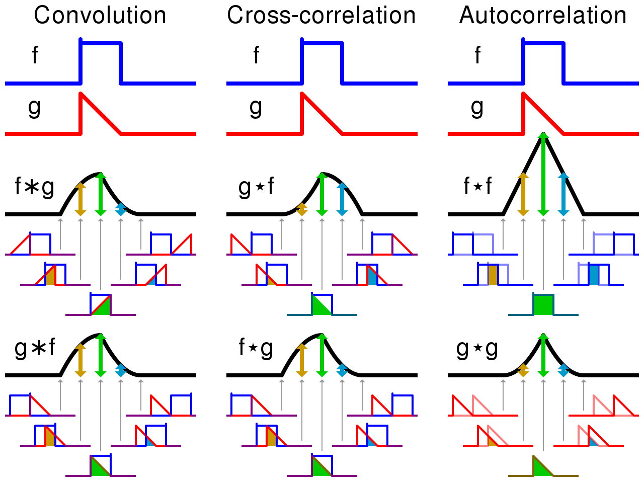
As I understand it (please correct me if I'm wrong), correlation can be used to see if one signal is a time-lagged copy of another signal (similar to how cosine and sine differ by a phase difference). So autocorrelation is testing a signal against itself to measure the times at which the time-lag repeats said signal. Using the example posted here:

result = np.correlate(x, x, mode='full')

Since x and t each consist of 100 elements and result consists of 199 elements, I am not sure why I should arbitrarily select the last 100 elements.

print("\n autocorrelation (shape={}):\n{}\n".format(result.shape, result))  

 autocorrelation (shape=(199,)):
[ 0.00000000e+00 -3.82130761e-16 -9.73648712e-02 -3.70014208e-01
 -8.59889695e-01 -1.56185995e+00 -2.41986054e+00 -3.33109112e+00
 -4.15799070e+00 -4.74662427e+00 -4.94918053e+00 -4.64762251e+00
 -3.77524157e+00 -2.33298717e+00 -3.97976240e-01  1.87752669e+00
  4.27722402e+00  6.54129270e+00  8.39434617e+00  9.57785701e+00
  9.88331103e+00  9.18204933e+00  7.44791758e+00  4.76948221e+00
  1.34963425e+00 -2.50822289e+00 -6.42666652e+00 -9.99116299e+00
 -1.27937834e+01 -1.44791297e+01 -1.47873668e+01 -1.35893098e+01
 -1.09091510e+01 -6.93157447e+00 -1.99159756e+00  3.45267493e+00
  8.86228186e+00  1.36707567e+01  1.73433176e+01  1.94357232e+01
  1.96463736e+01  1.78556800e+01  1.41478477e+01  8.81191526e+00
  2.32100171e+00 -4.70897483e+00 -1.15775811e+01 -1.75696560e+01
 -2.20296487e+01 -2.44327920e+01 -2.44454330e+01 -2.19677060e+01
 -1.71533510e+01 -1.04037163e+01 -2.33560966e+00  6.27458308e+00
  1.45655029e+01  2.16769872e+01  2.68391837e+01  2.94553896e+01
  2.91697473e+01  2.59122266e+01  1.99154591e+01  1.17007613e+01
  2.03381596e+00 -8.14633251e+00 -1.78184255e+01 -2.59814393e+01
 -3.17580589e+01 -3.44884934e+01 -3.38046447e+01 -2.96763956e+01
 -2.24244433e+01 -1.26974172e+01 -1.41464998e+00  1.03204331e+01
  2.13281784e+01  3.04712823e+01  3.67721634e+01  3.95170295e+01
  3.83356037e+01  3.32477037e+01  2.46710643e+01  1.33886439e+01
  4.77778141e-01 -1.27924775e+01 -2.50860560e+01 -3.51343866e+01
 -4.18671622e+01 -4.45258983e+01 -4.27482779e+01 -3.66140001e+01
 -2.66465884e+01 -1.37700036e+01  7.76494745e-01  1.55574483e+01
  2.90828312e+01  3.99582426e+01  4.70285203e+01  4.95000000e+01
  4.70285203e+01  3.99582426e+01  2.90828312e+01  1.55574483e+01
  7.76494745e-01 -1.37700036e+01 -2.66465884e+01 -3.66140001e+01
 -4.27482779e+01 -4.45258983e+01 -4.18671622e+01 -3.51343866e+01
 -2.50860560e+01 -1.27924775e+01  4.77778141e-01  1.33886439e+01
  2.46710643e+01  3.32477037e+01  3.83356037e+01  3.95170295e+01
  3.67721634e+01  3.04712823e+01  2.13281784e+01  1.03204331e+01
 -1.41464998e+00 -1.26974172e+01 -2.24244433e+01 -2.96763956e+01
 -3.38046447e+01 -3.44884934e+01 -3.17580589e+01 -2.59814393e+01
 -1.78184255e+01 -8.14633251e+00  2.03381596e+00  1.17007613e+01
  1.99154591e+01  2.59122266e+01  2.91697473e+01  2.94553896e+01
  2.68391837e+01  2.16769872e+01  1.45655029e+01  6.27458308e+00
 -2.33560966e+00 -1.04037163e+01 -1.71533510e+01 -2.19677060e+01
 -2.44454330e+01 -2.44327920e+01 -2.20296487e+01 -1.75696560e+01
 -1.15775811e+01 -4.70897483e+00  2.32100171e+00  8.81191526e+00
  1.41478477e+01  1.78556800e+01  1.96463736e+01  1.94357232e+01
  1.73433176e+01  1.36707567e+01  8.86228186e+00  3.45267493e+00
 -1.99159756e+00 -6.93157447e+00 -1.09091510e+01 -1.35893098e+01
 -1.47873668e+01 -1.44791297e+01 -1.27937834e+01 -9.99116299e+00
 -6.42666652e+00 -2.50822289e+00  1.34963425e+00  4.76948221e+00
  7.44791758e+00  9.18204933e+00  9.88331103e+00  9.57785701e+00
  8.39434617e+00  6.54129270e+00  4.27722402e+00  1.87752669e+00
 -3.97976240e-01 -2.33298717e+00 -3.77524157e+00 -4.64762251e+00
 -4.94918053e+00 -4.74662427e+00 -4.15799070e+00 -3.33109112e+00
 -2.41986054e+00 -1.56185995e+00 -8.59889695e-01 -3.70014208e-01
 -9.73648712e-02 -3.82130761e-16  0.00000000e+00]

Attempt 2: Fourier

Since I am not sure where to go from the last attempt, I sought a new attempt. To my understanding, Fourier analysis basically shifts a signal from/to the time-domain (x(t) vs t) to/from the frequency domain (x(t) vs f=1/t); the signal in frequency-space should appear as a sinusoidal wave that dampens over time. The period is obtained from the most observed frequency since this is the location of the peak of the distribution of frequencies.

Since my values are all real-valued, applying the Fourier transform should mean my output values are all complex-valued. I wouldn't think this is a problem, except for the fact that scipy has methods for real-values. I do not fully understand the differences between all of the different scipy methods. That makes following the algorithm proposed in this posted solution hard for me to follow (ie, how/why is the threshold value picked?).

omega = np.fft.fft(x)
freq = np.fft.fftfreq(x.size, 1)
threshold = 0
idx = np.where(abs(omega)>threshold)[0][-1]
max_f = abs(freq[idx])
print(max_f)

This outputs 0.01, meaning the period is 1/0.01 = 100. This doesn't make sense either.

Attempt 3: Power Spectral Density

According to the scipy docs, I should be able to estimate the power spectral density (psd) of the signal using a periodogram (which, according to wikipedia, is the fourier transform of the autocorrelation function). By selecting the dominant frequency fmax at which the signal peaks, the period of the signal can be obtained as 1 / fmax.

freq, pdensity = signal.periodogram(x)

fig, ax = plt.subplots()
ax.plot(freq, pdensity, color='r')
ax.grid(color='k', alpha=0.3, linestyle=':')
plt.show()
plt.close(fig)

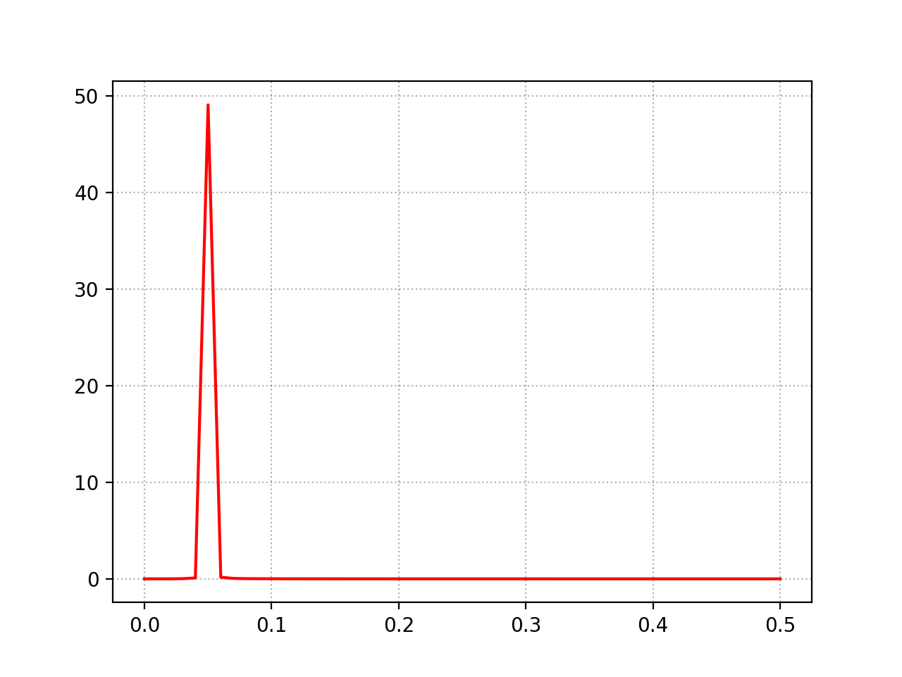
The periodogram shown below peaks at 49.076... at a frequency of fmax = 0.05. So, period = 1/fmax = 20. This doesn't make sense to me. I have a feeling it has something to do with the sampling rate, but don't know enough to confirm or progress further.

I realize I am missing some fundamental gaps in understanding how these things work. There are a lot of resources online, but it's hard to find this needle in the haystack. Can someone help me learn more about this?

Hayrack

Just a small comment to promote understanding of Attempt 1: if you look at the list of numbers output by the autocorrelation function, you'll notice that the 20th element has a peak value of 9.88331103. You'll also notice that your sine function has a period of ~20 samples. Ergo: the autocorrelation function is telling you that the period is about 20 samples long. – Psychological

Answer 1

Let's first look at your signal (I've added endpoint=False to make the division even):

t = np.linspace(0, 10*np.pi, 100, endpoint=False)
x = np.sin(t)

Let's divide out the radians (essentially by taking t /= 2*np.pi) and create the same signal by relating to frequencies:

fs = 20 # Sampling rate of 100/5 = 20 (e.g. Hz)
f = 1 # Signal frequency of 1 (e.g. Hz)
t = np.linspace(0, 5, 5*fs, endpoint=False)
x = np.sin(2*np.pi*f*t)

This makes it more salient that f/fs == 1/20 == 0.05 (i.e. the periodicity of the signal is exactly 20 samples). Frequencies in a digital signal always relate to its sampling rate, as you have already guessed. Note that the actual signal is exactly the same no matter what the values of f and fs are, as long as their ratio is the same:

fs = 1 # Natural units
f = 0.05
t = np.linspace(0, 100, 100*fs, endpoint=False)
x = np.sin(2*np.pi*f*t)

In the following I'll use these natural units (fs = 1). The only difference will be in t and hence the generated frequency axes.

Autocorrelation

Your understanding of what the autocorrelation function does is correct. It detects the correlation of a signal with a time-lagged version of itself. It does this by sliding the signal over itself as seen in the right column here (from Wikipedia):

Note that as both inputs to the correlation function are the same, the resulting signal is necessarily symmetric. That is why the output of np.correlate is usually sliced from the middle:

acf = np.correlate(x, x, 'full')[-len(x):]

Now index 0 corresponds to 0 delay between the two copies of the signal.

Next you'll want to find the index or delay that presents the largest correlation. Due to the shrinking overlap this will by default also be index 0, so the following won't work:

acf.argmax() # Always returns 0

Instead I recommend to find the largest peak instead, where a peak is defined to be any index with a larger value than both its direct neighbours:

inflection = np.diff(np.sign(np.diff(acf))) # Find the second-order differences
peaks = (inflection < 0).nonzero()[0] + 1 # Find where they are negative
delay = peaks[acf[peaks].argmax()] # Of those, find the index with the maximum value

Now delay == 20, which tells you that the signal has a frequency of 1/20 of its sampling rate:

signal_freq = fs/delay # Gives 0.05

Fourier transform

You used the following to calculate the FFT:

omega = np.fft.fft(x)
freq = np.fft.fftfreq(x.size, 1)

Thhese functions re designed for complex-valued signals. They will work for real-valued signals, but you'll get a symmetric output as the negative frequency components will be identical to the positive frequency components. NumPy provides separate functions for real-valued signals:

ft = np.fft.rfft(x)
freqs = np.fft.rfftfreq(len(x), t[1]-t[0]) # Get frequency axis from the time axis
mags = abs(ft) # We don't care about the phase information here

Let's have a look:

plt.plot(freqs, mags)
plt.show()

Note two things: the peak is at frequency 0.05, and the maximum frequency on the axis is 0.5 (the Nyquist frequency, which is exactly half the sampling rate). If we had picked fs = 20, this would be 10.

Now let's find the maximum. The thresholding method you have tried can work, but the target frequency bin is selected blindly and so this method would suffer in the presence of other signals. We could just select the maximum value:

signal_freq = freqs[mags.argmax()] # Gives 0.05

However, this would fail if, e.g., we have a large DC offset (and hence a large component in index 0). In that case we could just select the highest peak again, to make it more robust:

inflection = np.diff(np.sign(np.diff(mags)))
peaks = (inflection < 0).nonzero()[0] + 1
peak = peaks[mags[peaks].argmax()]
signal_freq = freqs[peak] # Gives 0.05

If we had picked fs = 20, this would have given signal_freq == 1.0 due to the different time axis from which the frequency axis was generated.

Periodogram

The method here is essentially the same. The autocorrelation function of x has the same time axis and period as x, so we can use the FFT as above to find the signal frequency:

pdg = np.fft.rfft(acf)
freqs = np.fft.rfftfreq(len(x), t[1]-t[0])

plt.plot(freqs, abs(pdg))
plt.show()

This curve obviously has slightly different characteristics from the direct FFT on x, but the main takeaways are the same: the frequency axis ranges from 0 to 0.5*fs, and we find a peak at the same signal frequency as before: freqs[abs(pdg).argmax()] == 0.05.

Edit:

To measure the actual periodicity of np.sin, we can just use the "angle axis" that we passed to np.sin instead of the time axis when generating the frequency axis:

freqs = np.fft.rfftfreq(len(x), 2*np.pi*f*(t[1]-t[0]))
rad_period = 1/freqs[mags.argmax()] # 6.283185307179586

Though that seems pointless, right? We pass in 2*np.pi and we get 2*np.pi. However, we can do the same with any regular time axis, without presupposing pi at any point:

fs = 10
t = np.arange(1000)/fs
x = np.sin(t)
rad_period = 1/np.fft.rfftfreq(len(x), 1/fs)[abs(np.fft.rfft(x)).argmax()] # 6.25

Naturally, the true value now lies in between two bins. That's where interpolation comes in and the associated need to choose a suitable window function.

Ritchie

Thank you for the very detailed response! As a follow-up to one of your points, you mention the large DC offset could alter the maximum frequency obtained from the signal. So by this logic, can I place mags -= mags[0] before calling signal_freq = freqs[mags.argmax()] # Gives 0.05? – Hayrack

Yes, there are ways you can remove this offset. Your suggestion would shift the entire FFT down, though—instead you should just zero out the first bin mags[0] = 0. Another way would be to do np.fft.rfft(x - x.mean()) which should also remove most DC bias. – Ritchie

So in choosing a particular method, I would imagine autocorrelation may require signals with very little noise, whereas fourier frequency decomposition is generally safer. Is this correct? – Hayrack

I wouldn't say the autocorrelation is particularly sensitive to noise, but it is sensitive to other frequency components. If you have multiple superimposed signals, this time-domain analysis becomes unreliable. That's where Fourier analysis shines, as it separates out the individual frequency components. – Ritchie

By the way, in this example we have a nice even fs/f == 20 which is why we were able to find the frequency exactly. In the general case, the desired frequency will be in between two delays (in the ACF) or bins (in the FFT or periodogram). When that happens, you'll want to interpolate between them to find the precise value. Things like windowing functions will become quite important then. – Ritchie

Sorry for so many questions. My last follow-up is: given all this, how does one numerically get that the period of oscillations is 2 pi? – Hayrack

Actually see my edit, I've added a bit more information on that. – Ritchie