There are many possible reasons for that. As benjaminplanche stated you need to use .mean instead of .sum reduction. Also, KLD term weight could be different for different architecture and data sets. So, try different weights and see the reconstruction loss, and latent space to decide. There is a trade-off between reconstruction loss (output quality) and KLD term which forces the model to shape a gausian like latent space.
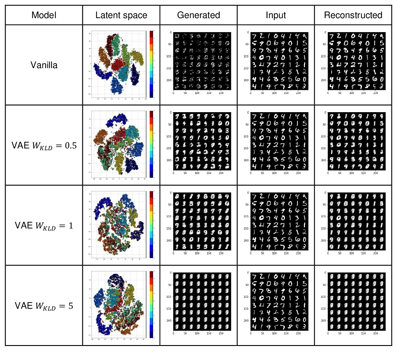
To evaluate different aspects of VAEs I trained a Vanilla autoencoder and VAE with different KLD term weights.
Note that, I used the MNIST hand-written digits dataset to train networks with input size 784=28*28 and latent size 30 dimensions. Although for data samples in range of [0, 1] we normally use a Sigmoid activation function, I used a Tanh for experimental reasons.
Vanilla Autoencoder:
Autoencoder(
  (encoder): Encoder(
    (nn): Sequential(
      (0): Linear(in_features=784, out_features=30, bias=True)
    )
  )
  (decoder): Decoder(
    (nn): Sequential(
      (0): Linear(in_features=30, out_features=784, bias=True)
      (1): Tanh()
    )
  )
)
Afterward, I implemented the VAE model as shown in the following code blocks. I trained this model with different KLD weights from the set {0.5, 1, 5}.
class VAE(nn.Module):

    def __init__(self,dim_latent_representation=2):

        super(VAE,self).__init__()

        class Encoder(nn.Module):
            def __init__(self, output_size=2):
                super(Encoder, self).__init__()
                # needs your implementation
                self.nn = nn.Sequential(
                nn.Linear(28 * 28, output_size),
                )

            def forward(self, x):
                # needs your implementation
                return self.nn(x)

        class Decoder(nn.Module):
            def __init__(self, input_size=2):
                super(Decoder, self).__init__()
                # needs your implementation
                self.nn = nn.Sequential(
                nn.Linear(input_size, 28 * 28),
                nn.Tanh(),
                )

            def forward(self, z):
                # needs your implementation
                return self.nn(z)

        self.dim_latent_representation = dim_latent_representation
        self.encoder = Encoder(output_size=dim_latent_representation)
        self.mu_layer = nn.Linear(self.dim_latent_representation, self.dim_latent_representation)
        self.logvar_layer = nn.Linear(self.dim_latent_representation, self.dim_latent_representation)
        self.decoder = Decoder(input_size=dim_latent_representation)
    # Implement this function for the VAE model
    def reparameterise(self, mu, logvar):

        if self.training:
            std = logvar.mul(0.5).exp_()
            eps = std.data.new(std.size()).normal_()
            return eps.mul(std).add_(mu)
        else:
            return mu

    def forward(self,x):

        # This function should be modified for the DAE and VAE
        x = self.encoder(x)
        mu, logvar = self.mu_layer(x), self.logvar_layer(x)
        z = self.reparameterise(mu, logvar)
        return self.decoder(z), mu, logvar
Here you can see output results from different models. I also visualized the 30 dimensional latent space in 2D using sklearn.manifold.TSNE transformation.
![enter image description here]()
We observe a low loss value for the vanilla autoencoder with 30D bottleneck size which results in high-quality reconstructed images. Although loss values increased in VAEs, the VAE arranged the latent space such that gaps between latent representations for different classes decreased. It means we can get better manipulated (mixed latents) output. Since VAE follows an isotropic multivariate normal distribution at the latent space, we can generate new unseen images by taking samples from the latent space with higher quality compared to the Vanilla autoencoder. However, the reconstruction quality was reduced (loss values increased) since the loss function is a weighted combination of MSE and KLD terms to be optimized where the KLD term forces the latent space to resemble a Gaussian distribution. As we increased the KLD weight, we achieved a more compact latent space closer to the prior distribution by sacrificing the reconstruction quality.


