How to add boundary constraints to a spline with geomdl or other library?
Asked Answered
G

1

0

Here is the spline without constraints:

from geomdl import fitting
from geomdl.visualization import VisMPL
path =  [(2077.0, 712.0, 1136.6176470588234), (2077.0004154771536, 974.630482962754, 1313.735294117647), (2077.1630960823995, 1302.460574562254, 1490.8529411764707), (2078.1944091179635, 1674.693193015173, 1667.9705882352941), (2080.5096120056783, 2086.976611915444, 1845.0882352941176), (2085.1051468332066, 2711.054258877495, 2022.2058823529412), (1477.0846185328733, 2803.6223679691457, 2199.323529411765), (948.4693105162195, 2802.0390667447105, 2376.4411764705883), (383.8615403256207, 2804.843424134807, 2553.5588235294117), (-41.6669725172834, 2497.067373170676, 2730.676470588235), (-37.94311919744064, 1970.5155845437525, 2907.794117647059), (-35.97395938535092, 1576.713103381243, 3084.9117647058824), (-35.125016151504795, 1214.2319876178394, 3262.029411764706), (-35.000550767864524, 893.3910350913443, 3439.1470588235297), (-35.0, 631.2108462417168, 3616.264705882353), (-35.0, 365.60545190581837, 3793.3823529411766), (-35.0, 100.00005756991993, 3970.5)]
degree = 3
curve = fitting.interpolate_curve(path, degree)
curve.vis = VisMPL.VisCurve3D()
curve.render()
# the following is to show it under matplotlib and prepare solutions comparison
import numpy as np
import matplotlib.pyplot as plt
qtPoints = 3*len(path)
s = np.linspace(0, 1, qtPoints, True).tolist()
pt = curve.tangent(s) # returns points and tangents
spline = [u for u, v in pt] # get points, leave tangents

enter image description here

I want to add constraints:

  • x >= -35
  • x <= 2077
  • y <= 2802

The geomdl library does not propose splines with constraints. I have tried this hack, just by correcting points to stay inside the boundaries:

path2 = [(x if x >= -35 else -35, y if y <= 2802 else 2802, z) for x,y,z in spline]
path2 = [(x if x <= 2077 else 2077, y, z) for x,y,z in path2]
curve2 = fitting.interpolate_curve(path2, 3)
pt2 = curve2.tangent(s) # returns points and tangents
spline2 = [u for u, v in pt2] # get points, leave tangents
plt.plot([u[0] for u in path], [u[1] for u in path], 'o', 
    [u[0] for u in spline], [u[1] for u in spline], 'b',
    [u[0] for u in spline2], [u[1] for u in spline2], 'r')
plt.show()

curve2.vis = VisMPL.VisCurve3D()
curve2.render()

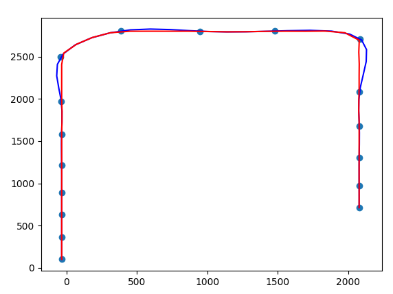
enter image description here

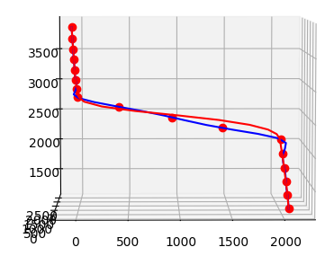
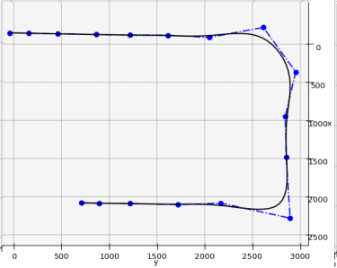
Here are both together (turned 90° left):

enter image description here

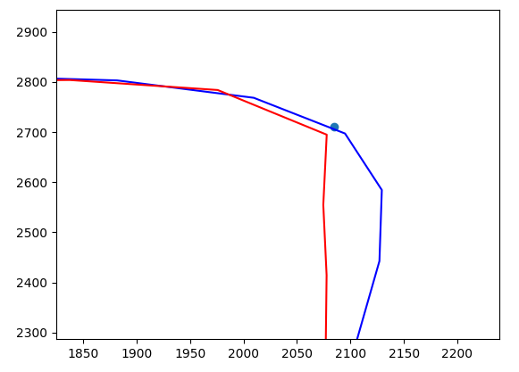
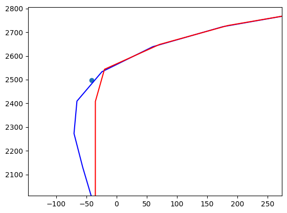
The result is not satisfactory (in red):

enter image description here

enter image description here

Another way is to use directly the path as control points. Here is the result with NURBS:

from geomdl import NURBS
curve_n = NURBS.Curve()
curve_n.degree = min(degree, len(path)) # order = degree+1
curve_n.ctrlpts = path
last_knot = len(path) - curve_n.degree
curve_n.knotvector = np.concatenate((np.zeros(curve_n.degree), np.arange(0, last_knot + 1), np.ones(curve_n.degree)*last_knot)).astype(int)
curve_n.delta = 0.05
spline_n = curve_n.evalpts
plt.plot([u[0] for u in path], [u[1] for u in path], 'o', 
    [u[0] for u in spline_f], [u[1] for u in spline_f], 'b',
    [u[0] for u in spline2], [u[1] for u in spline2], 'r',
    [u[0] for u in spline_n], [u[1] for u in spline_n], 'g')
plt.show()

enter image description here

The result (in green) is too far from the path.

If I use the NURBS points to perform a new fitting, and playing with the NURBS degree, I obtain something satisfactory:

from geomdl import fitting
from geomdl import NURBS
#from geomdl.visualization import VisMPL
import numpy as np
import matplotlib.pyplot as plt
path =  [(2077.0, 712.0, 1136.6176470588234), (2077.0004154771536, 974.630482962754, 1313.735294117647), (2077.1630960823995, 1302.460574562254, 1490.8529411764707), (2078.1944091179635, 1674.693193015173, 1667.9705882352941), (2080.5096120056783, 2086.976611915444, 1845.0882352941176), (2085.1051468332066, 2711.054258877495, 2022.2058823529412), (1477.0846185328733, 2803.6223679691457, 2199.323529411765), (948.4693105162195, 2802.0390667447105, 2376.4411764705883), (383.8615403256207, 2804.843424134807, 2553.5588235294117), (-41.6669725172834, 2497.067373170676, 2730.676470588235), (-37.94311919744064, 1970.5155845437525, 2907.794117647059), (-35.97395938535092, 1576.713103381243, 3084.9117647058824), (-35.125016151504795, 1214.2319876178394, 3262.029411764706), (-35.000550767864524, 893.3910350913443, 3439.1470588235297), (-35.0, 631.2108462417168, 3616.264705882353), (-35.0, 365.60545190581837, 3793.3823529411766), (-35.0, 100.00005756991993, 3970.5)]
degree = 3
qtPoints = 3*len(path)

# fitting without constraints
curve_f = fitting.interpolate_curve(path, degree)
#curve.vis = VisMPL.VisCurve3D()
#curve.render()
s = np.linspace(0, 1, qtPoints, True).tolist()
pt = curve_f.tangent(s) # returns points and tangents
spline  = [u for u, v in pt] # get points, leave tangents

# fitting with constraints, awkward hack
path2 = [(x if x >= -35 else -35, y if y <= 2802 else 2802, z) for x,y,z in spline]
path2 = [(x if x <= 2077 else 2077, y, z) for x,y,z in path2]
curve2 = fitting.interpolate_curve(path2, 3)
pt2 = curve2.tangent(s) # returns points and tangents
spline2 = [u for u, v in pt2] # get points, leave tangents

# control points = path
curve_n = NURBS.Curve()
curve_n.degree = 2 #min(degree, len(path)) # order = degree+1
curve_n.ctrlpts = path
last_knot = len(path) - curve_n.degree
curve_n.knotvector = np.concatenate((np.zeros(curve_n.degree), np.arange(0, last_knot + 1), np.ones(curve_n.degree)*last_knot)).astype(int)
curve_n.delta = 0.05
spline_n = curve_n.evalpts

# fitting without constraints on NURBS points
curve3 = fitting.interpolate_curve(spline_n, 3)
pt3 = curve3.tangent(s) # returns points and tangents
spline3 = [u for u, v in pt3] # get points, leave tangents

plt.plot([u[0] for u in path], [u[1] for u in path], 'o', 
    [u[0] for u in spline_f], [u[1] for u in spline_f], 'b',
    [u[0] for u in spline2], [u[1] for u in spline2], 'r',
    [u[0] for u in spline3], [u[1] for u in spline3], 'y',
    [u[0] for u in spline_n], [u[1] for u in spline_n], 'g')
plt.show()

enter image description here

But it is not robust, and possibly just an infamous DIY.

[True if x >= -35 and x <= 2077 and y <= 2802 else False for x,y,z in spline3]
[True, False, False, False, False, False, False, False, False, False, False, False, False, False, True, True, True, True, True, True, True, False, False, False, False, True, True, True, True, True, True, True, True, False, False, False, False, False, False, False, False, False, False, False, False, True, False, False, True, True, True]

How to keep it smooth, on the path, and whith respect to the constraints please, possibly with another library? I found this, but that solves derivatives constraints and I don't figure out how to adapt this solution. I raised also the question on a strictly mathematical point of view here.

Gristly answered 8/5, 2020 at 7:55 Comment(2)
@askewchan, that may be for youGristly
@AlexI, that may be for you tooGristly
G
1

Well, tough topic, but I got it, inspired by this for 2D border (derivative) constrained splines. The proposed solution makes use also of scipy.optimize.minimize.

Here is the full code, and after some explanations:

import numpy as np
from scipy.interpolate import UnivariateSpline, splev, splprep, BSpline
from scipy.optimize import minimize

xmin = -35
xmax = 2077
ymax = 2802

def guess(p, k, s, w=None):
    """Do an ordinary spline fit to provide knots"""
    return splprep(p, w, k=k, s=s)

def err(c, p, u, t, c_shape, k, w=None):
    """The error function to minimize"""
    diff = (np.array(p) - splev(u, (t, c.reshape(c_shape), k))).flatten()
    if w is None:
        diff = (diff*diff).sum()
    else:
        diff = (diff*diff*w).sum() #not sure it is the good way to multiply w
    return np.abs(diff)

def constraint(c, l, t, c_shape, k, eqorineq, eqinterv):
    X = np.linspace(0, 1, l*20)
    v = splev(X, (t, c.reshape(c_shape), k))
    if eqorineq == 'ineq':
        ineq_contrib =  sum([(x < xmin)*(x-xmin)**2 + (x > xmax)*(x-xmax)**2 for x in v[0]] \
            + [(y > ymax)*(y-ymax)**2 for y in v[1]])
        eq_contrib = 0
        for i in range(len(X)):
            eq_contrib += (X[i] >= eqinterv[0][0] and X[i] <= eqinterv[0][1]) * (v[0][i] - xmin)**2 \
                + (X[i] >= eqinterv[1][0] and X[i] <= eqinterv[1][1]) * (v[0][i] - xmax)**2 \
                + (X[i] >= eqinterv[2][0] and X[i] <= eqinterv[2][1]) * (v[1][i] - ymax)**2
        return -(ineq_contrib + eq_contrib)
#        return -1 * ineq_contrib
    elif eqorineq == 'eq':
        res = 0 # equality
        for i in range(len(X)):
            if X[i] >= eqinterv[0][0] and X[i] <= eqinterv[0][1] and v[0][i] != xmin \
                or X[i] >= eqinterv[1][0] and X[i] <= eqinterv[1][1] and v[0][i] != xmax \
                or X[i] >= eqinterv[2][0] and X[i] <= eqinterv[2][1] and v[1][i] != ymax :
                res = 1
        return res

def spline_neumann(p, k=3, s=0, w=None):
    tck, u = guess(p, k, s, w=w)
    t, c0, k = tck
    c0flat = np.array(c0).flatten()
    c_shape = np.array(c0).shape
    x0 = 0 #x[0] # point at which zero slope is required

    # compute u intervals for eq constraints
    xmin_umin = xmin_umax = xmax_umin = xmax_umax = ymax_umin = ymax_umax = -1
    for i in range(len(p[0])):
        if xmin_umin == -1 and p[0][i] <= xmin : xmin_umin = u[i] 
        if xmin_umin != -1 and xmin_umax == -1 and p[0][i] > xmin : xmin_umax = u[i-1] 
        if xmax_umin == -1 and p[0][i] >= xmax : xmax_umin = u[i] 
        if xmax_umin != -1 and xmax_umax == -1 and p[0][i] < xmax : xmax_umax = u[i-1] 
        if ymax_umin == -1 and p[1][i] >= ymax : ymax_umin = u[i] 
        if ymax_umin != -1 and ymax_umax == -1 and p[1][i] < ymax : ymax_umax = u[i-1] 
    eqinterv = [[xmin_umin, xmin_umax], [xmax_umin, xmax_umax], [ymax_umin, ymax_umax]]
    for i in range(len(eqinterv)):
        if eqinterv[i][0] == -1 : eqinterv[i][0] = 0
        if eqinterv[i][1] == -1 : eqinterv[i][1] = 1
    print("eqinterv = ", eqinterv)

    con = {'type': 'ineq', 'fun': lambda c: constraint(c, len(p[0]), t, c_shape, k, 'ineq', eqinterv)
           #'type': 'eq', 'fun': lambda c: constraint(c, len(p[0]), t, c_shape, k, 'eq', eqinterv)
           #'fun': lambda c: splev(x0, (t, c.reshape(c_shape), k), der=1),
           #'jac': lambda c: splev(x0, (t, c, k), der=2) # doesn't help, dunno why
           }
    opt = minimize(err, c0flat, (p, u, t, c_shape, k, w), constraints=con)
    #opt = minimize(err, c0, (p, u, t, c_shape, k, w), method='Nelder-Mead', constraints=con)
    #opt = minimize(err, c0flat, (p, u, t, c_shape, k, w))
    copt = opt.x.reshape(c_shape)
    #return UnivariateSpline._from_tck((t, copt, k))
    #return BSpline(t, k, copt)
    return ((t, copt, k), opt.success)

import matplotlib.pyplot as plt

path =  [(2077.0, 712.0, 1136.6176470588234), (2077.0004154771536, 974.630482962754, 1313.735294117647), (2077.1630960823995, 1302.460574562254, 1490.8529411764707), (2078.1944091179635, 1674.693193015173, 1667.9705882352941), (2080.5096120056783, 2086.976611915444, 1845.0882352941176), (2085.1051468332066, 2711.054258877495, 2022.2058823529412), (1477.0846185328733, 2803.6223679691457, 2199.323529411765), (948.4693105162195, 2802.0390667447105, 2376.4411764705883), (383.8615403256207, 2804.843424134807, 2553.5588235294117), (-41.6669725172834, 2497.067373170676, 2730.676470588235), (-37.94311919744064, 1970.5155845437525, 2907.794117647059), (-35.97395938535092, 1576.713103381243, 3084.9117647058824), (-35.125016151504795, 1214.2319876178394, 3262.029411764706), (-35.000550767864524, 893.3910350913443, 3439.1470588235297), (-35.0, 631.2108462417168, 3616.264705882353), (-35.0, 365.60545190581837, 3793.3823529411766), (-35.0, 100.00005756991993, 3970.5)]
pathxyz = [[x for x,y,z in path], [y for x,y,z in path], [z for x,y,z in path]]
n = len(path)
#std would be interesting to define as the standard deviation of the curve compared to a no noise one. No noise ==> s=0
k = 5
s = 0
sp0, u = guess(pathxyz, k, s)
sp, success = spline_neumann(pathxyz, k, s) #s=n*std
print("success = ", success)
# % of points not respecting the constraints
perfo_vs_ineq = (sum([(x < xmin) for x in v[0]]) + sum([(x > xmax) for x in v[0]]) + sum([(y > ymax) for y in v[1]]) )/len(v[0])/2
print("perfo% vs ineq constraints = ", perfo_vs_ineq)

X = np.linspace(0, 1, len(pathxyz)*10)
val0 = splev(X, sp0)
val = splev(X, sp)

fig = plt.figure()
ax = fig.gca(projection='3d')
ax.plot([x for x,y,z in path], [y for x,y,z in path], [z for x,y,z in path], 'ro')
ax.plot(val0[0], val0[1], val0[2], 'b-')
ax.plot(val[0], val[1], val[2], 'r-')
plt.show()

plt.figure()
plt.plot(val0[0], val0[1], '-b', lw=1, label='guess')
plt.plot(val[0], val[1], '-r', lw=2, label='spline')
plt.plot(pathxyz[0], pathxyz[1], 'ok', label='data')
plt.legend(loc='best')
plt.show()

At the end, I have both a 2D and 3D rendering. The 3D view shows that the spline uses the z-axes for smoothing. That's not satisfactory for my use case, so I will have to take it into account in my constraints, but that's out of the scope of this Q/A:

enter image description here

enter image description here

And the 2D view that shows the constraints effects on the spline:

enter image description here

The blue curve is without constraints, and the red one with.

Now the explanations for the wayforward:

  • The spline without constraints is computed with: sp0, u = guess(pathxyz, k, s)
  • The spline with constraints is computed with: sp, success = spline_neumann(pathxyz, k, s)
  • Then it prints success following scipy.optimize.minimize criteria and a custom criteria based on inequalities constraints as the percentage of points not satisfying the constraints:
    print("success = ", success)
    perfo_vs_ineq = (sum([(x < xmin) for x in v[0]]) + sum([(x > xmax) for x in v[0]]) + sum([(y > ymax) for y in v[1]]) )/len(v[0])/2
    print("perfo% vs ineq constraints = ", perfo_vs_ineq)
  • The optimisation under constraints is performed by: opt = minimize(err, c0flat, (p, u, t, c_shape, k, w), constraints=con). It optimises the coefficients of the spline initialised with c0flat obtained by the non constrained solving
  • It returns the coefficients in copt = opt.x we have to reshape to be able to be used by splev with copt = opt.x.reshape(c_shape)
  • splev is used to evaluate both splines - unconstrained and constrained - nothing new here:
X = np.linspace(0, 1, len(pathxyz)*10)
val0 = splev(X, sp0)
val = splev(X, sp)
  • The scipy.optimize.minimize arguments and return values are explained in the manual. So I am going to explain only what is specific here
  • err is the cost to minimize. It is built to stick to the control points:
def err(c, p, u, t, c_shape, k, w=None):
    """The error function to minimize"""
    diff = (np.array(p) - splev(u, (t, c.reshape(c_shape), k))).flatten()
    if w is None:
        diff = (diff*diff).sum()
    else:
        diff = (diff*diff*w).sum() #not sure it is the good way to multiply w
    return np.abs(diff)
  • I have not tested with the weight argument w. What's important to understand here is that we perform the evaluation on the control points only, using the curvilinear coordinates provided by u. The cost is the difference between the control points and how they are evaluated with the new computed coefficients c tried by scipy.optimize.minimize
  • And then we come to the constraints provided to scipy.optimize.minimize by constraints=con defined as:
    con = {'type': 'ineq', 'fun': lambda c: constraint(c, len(p[0]), t, c_shape, k, 'ineq', eqinterv)
           #'type': 'eq', 'fun': lambda c: constraint(c, len(p[0]), t, c_shape, k, 'eq', eqinterv)
  • I use only inequalities since tests with equalities gives poor results in my use case, but I have let the code if it may help someone. So both inequalities and equalities constraints are computed with the function constraint(c, len(p[0]), t, c_shape, k, 'ineq', eqinterv). I have prefered one function instead of a list of ones to perform the spline evaluation only once. So of course, c is the argument under evaluation by scipy.optimize.minimize, t and k complete the (t,c,k) tuple required for evaluation, len(p[0]) is related to the number of points to evaluate which is proportional, 'ineq' tells constraint to deal with inequalities, and eqinterv is a vector where I want to evaluate equalities computed as a cost. In my use case, I recall I need x >= -35 and x <= 2077 and y <= 2802. I don't detail the calculation which is specific to my use case, I only stress the point the intervals are related to the curvilinear coordinates homogeneous to u:
    xmin_umin = xmin_umax = xmax_umin = xmax_umax = ymax_umin = ymax_umax = -1
    for i in range(len(p[0])):
        if xmin_umin == -1 and p[0][i] <= xmin : xmin_umin = u[i] 
        if xmin_umin != -1 and xmin_umax == -1 and p[0][i] > xmin : xmin_umax = u[i-1] 
        if xmax_umin == -1 and p[0][i] >= xmax : xmax_umin = u[i] 
        if xmax_umin != -1 and xmax_umax == -1 and p[0][i] < xmax : xmax_umax = u[i-1] 
        if ymax_umin == -1 and p[1][i] >= ymax : ymax_umin = u[i] 
        if ymax_umin != -1 and ymax_umax == -1 and p[1][i] < ymax : ymax_umax = u[i-1] 
  • Then the cost for equalities is computed with:
        eq_contrib = 0
        for i in range(len(X)):
            eq_contrib += (X[i] >= eqinterv[0][0] and X[i] <= eqinterv[0][1]) * (v[0][i] - xmin)**2 \
                + (X[i] >= eqinterv[1][0] and X[i] <= eqinterv[1][1]) * (v[0][i] - xmax)**2 \
                + (X[i] >= eqinterv[2][0] and X[i] <= eqinterv[2][1]) * (v[1][i] - ymax)**2
  • Inequalities cost is simple:
        ineq_contrib =  sum([(x < xmin)*(x-xmin)**2 + (x > xmax)*(x-xmax)**2 for x in v[0]] \
            + [(y > ymax)*(y-ymax)**2 for y in v[1]])

That's it, hoping it is usefull.

Gristly answered 9/5, 2020 at 9:9 Comment(0)

© 2022 - 2024 — McMap. All rights reserved.