Vlookup using 2 columns to reference another

Question

I am trying to do a vlookup under a circumstance of first then last name to get an age. This will be done within Column A, then Column B. If found in Column A, Continue to Column B, If found in Column B, put age in J3 that comes from Column C else put "None".

Here is an example:

J1 = John
J2 = Doe
J3 = =VLOOKUP J1 & J2,A1:C50,3,FALSE)

J3 is what I have so far. Do I need to nest a Vlookup to check Column A, then Column B in order to get the age?

Here is an example of the table list:

A     B    C
Jeff  Vel  80
John  Fly  25
Jake  Foo  20
John  Doe  55

J3 = 55.

Winner

Since you are looking up a number from a list, you could use =SUMIFS(C:C, A:A, J1, B:B, J2) assuming that your names are unique. You could also create a third column that concatenates the names then do a lookup on that. Inset C as a new column C1 (and copy down) =A1&B1. Then in J3 =vlookup(J1&J2, C:C, 2, false). – Balm

See Excel: match two columns and output third … AND… there are multiple instances in each column – Foreleg

@Jeeped why not Mjölnir this thread? – Kimbrough

@Balm , you might want to test that VLOOKUP... ,C:C,2 won't work – Hunkydory

Instead of relying on me coming back to post a follow up comment to fix it, some guidance for OP would be appreciated, @callumDA. Brad, my vlookup will fail because the table_array parameter should be C:D not C:C. – Balm

@ScottCraner - That link I pointed to is one of my best examples for this situation but has no magical unicorn farts. You cannot nuke a question as duplicate by pointing to an answer that has no magical unicorn farts and I don't feel like doing more research than the OP. – Foreleg

@Jeeped okay, so let's make one. Feel free to add to the answer below. – Kimbrough

@ScottCraner - Hrrumph... I was phishing for an upvote on the linked answer. That didn't work out! – Foreleg

@Jeeped my bad meant to do so, and got preoccupied. – Kimbrough

@JNevill. Apologies for the short answer. I would usually post the correction rather than just highlight the error. It might have something to do with the fact that I was on my phone with no access to Excel. However, I do feel like posting comments which are essentially answers can sometimes be an excuse for one to not test their suggestions properly. I think your comment should definitely have been an answer and in the process of writing up your answer you might have caught that error yourself. – Hunkydory

Answer 1

Many ways:

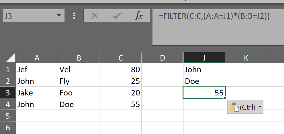
If one has the new Dynamic array formulas:

=FILTER(C:C,(A:A=J1)*(B:B=J2))

If not then:

1. Dealing with Number returns:

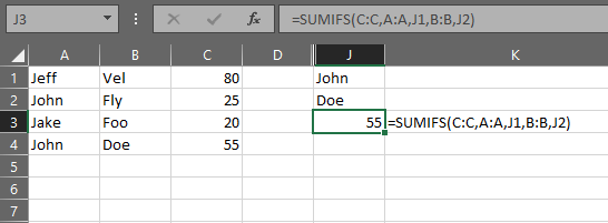
If your return values are numbers and the match is unique(there is only one John Doe in the data) or you want to sum the returns if there are multiples, then Using SUMIFS is the quickest method.

=SUMIFS(C:C,A:A,J1,B:B,J2)

---

2. With non numeric returns

If the returns are not numeric or there are multiples then there are two methods to get the first match in the list:

a. A helper column:

In a forth column put the following formula:

=A1&B1

and copy down the list

Then use INDEX/MATCH:

=INDEX(C:C,MATCH(J1&J2,D:D,0))

b. The array formula:

If you do not want or cannot create the forth column then use an array type formula:

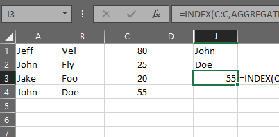
=INDEX(C:C,AGGREGATE(15,6,ROW($A$1:$A$4)/(($A$1:$A$4=J1)*($B$1:$B$4=J2)),1))

Array type formulas need to limit the size of the data to the data set.

If your data set changes sizes regularly we can modify the above to be dynamic by adding more INDEX/MATCH to return the last cell with data:

=INDEX(C:C,AGGREGATE(15,6,ROW($A$1:INDEX($A:$A,MATCH("ZZZ",A:A)))/(($A$1:INDEX($A:$A,MATCH("ZZZ",A:A))=J1)*($B$1:INDEX($B:$B,MATCH("ZZZ",A:A))=J2)),1))

This will allow the data set to grow or shrink and the formula will only iterate through those that have data and not the full column.

The methods described above are set in the order of Best-Better-Good.

---

3. To get multiple answers in one cell

If you do not want to sum, or the return values are text and there are multiple instances of John Doe and you want all the values returned in one cell then:

a. If you have Office 365 Excel you can use an array form of TEXTJOIN:

=TEXTJOIN(",",TRUE,IF(($A$1:$A$4=J1)*($B$1:$B$4=J2),$C$1:$C$4,""))

Being an array formula it needs to be confirmed with Ctrl-Shift-Enter instead of Enter when exiting edit mode. If done correctly then Excel will put {} around the formula.

Like the AGGREGATE formula above it needs to be limited to the data set. The ranges can be made dynamic with the INDEX/MATCH functions like above also.

b. If one does not have Office 365 Excel then add this code to a module attached to the workbook:

Function TEXTJOIN(delim As String, skipblank As Boolean, arr)
    Dim d As Long
    Dim c As Long
    Dim arr2()
    Dim t As Long, y As Long
    t = -1
    y = -1
    If TypeName(arr) = "Range" Then
        arr2 = arr.Value
    Else
        arr2 = arr
    End If
    On Error Resume Next
    t = UBound(arr2, 2)
    y = UBound(arr2, 1)
    On Error GoTo 0

    If t >= 0 And y >= 0 Then
        For c = LBound(arr2, 1) To UBound(arr2, 1)
            For d = LBound(arr2, 1) To UBound(arr2, 2)
                If arr2(c, d) <> "" Or Not skipblank Then
                    TEXTJOIN = TEXTJOIN & arr2(c, d) & delim
                End If
            Next d
        Next c
    Else
        For c = LBound(arr2) To UBound(arr2)
            If arr2(c) <> "" Or Not skipblank Then
                TEXTJOIN = TEXTJOIN & arr2(c) & delim
            End If
        Next c
    End If
    TEXTJOIN = Left(TEXTJOIN, Len(TEXTJOIN) - Len(delim))
End Function

Then use the TEXTJOIN() formula as described above.

Kimbrough

I really liked the use of SUMIFS. Simple yet innovative. I learned something. – Thermo

Answer 2

This is an alternative using VBA in a UDF

---

Based on this answer

---

This is a generic User Defined Function (UDF)

Steps

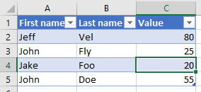
1. Add your data to an Excel structured table

2. Add this function to a Module

Code:

Public Function lookupValues(ByVal table As Range, ByVal criteria1_header As String, ByVal lookup_criteria1 As String, ByVal criteria2_header As String, ByVal lookup_criteria2 As String, ByVal return_header As String) As Variant
       
    On Error GoTo CleanFail
    
    ' Get criteria 1 column number from headers
    Dim criteria1Column As Long
    criteria1Column = Application.Match(criteria1_header, table.ListObject.HeaderRowRange, False)
    
    ' Get criteria 2 column number from headers
    Dim criteria2Column As Long
    criteria2Column = Application.Match(criteria2_header, table.ListObject.HeaderRowRange, False)
    
    ' Get value column number from headers according to function parameter
    Dim returnColumn As Long
    returnColumn = Application.Match(return_header, table.ListObject.HeaderRowRange, False)
    
    
    ' Get criteria 1 column values into 1d array
    Dim criteria1Values As Variant
    criteria1Values = WorksheetFunction.Transpose(Application.Index(table.Columns(criteria1Column), 0, 1))
    
    ' Get criteria 2 column values into 1d array
    Dim criteria2Values As Variant
    criteria2Values = WorksheetFunction.Transpose(Application.Index(table.Columns(criteria2Column), 0, 1))
    
    ' Define and redimension an array to hold the concatenated criteria 1 and criteria 2 values
    Dim criteria1_2Values() As Variant
    ReDim criteria1_2Values(1 To UBound(criteria1Values))
    
    ' Concatenate the criteria 1 and criteria 2 values and store them in an array
    Dim counter As Long
    For counter = 1 To UBound(criteria1Values)
        criteria1_2Values(counter) = criteria1Values(counter) & "|" & criteria2Values(counter)
    Next counter
    
    ' Get the matching row according to lookup values
    Dim resultRow As Variant
    resultRow = Application.Match(lookup_criteria1 & "|" & lookup_criteria2, criteria1_2Values, False)
    
    ' Get the result value according to the value column number
    Dim result As Variant
    result = Application.Index(table.Columns(returnColumn), resultRow)
    
    ' Return the value
CleanExit:
    lookupValues = result
    Exit Function
    
CleanFail:
    result = "Check function parameters"
    GoTo CleanExit
End Function

3. Call the function like this:

=lookupValues(TableName;E1;F1;E2;F2;E3)

Nonbeliever