Count Unique values with a condition

Question

In column A I have list of different names. In column B, I have values either 0 or 1.

I want to get a count of all the unique names from column A which have 1 in column B.

Using below array formula I am able count unique names but not able to apply condition on column B.

=SUM(1/COUNTIF(A:A,A:A))

Pediment

Answer 1

Assuming no more than 100 rows try this "array formula" to count the different names in A2:A100 where there is a 1 in the same row in B2:B100:

=SUM(IF(FREQUENCY(IF(B2:B100=1,IF(A2:A100<>"",MATCH(A2:A100,A2:A100,0))),ROW(A2:A100)-ROW(A2)+1),1))

confirmed with CTRL+SHIFT+ENTER

Note that I say different not unique as the two are not the same

Chassis

+ 1 Beat me to it by 5 secs :) – Obnoxious

Answer 2

Like this?

=SUM(--(FREQUENCY(IF(($B$1:$B$8=1), COUNTIF($A$1:$A$8, "<"&$A$1:$A$8), ""), COUNTIF($A$1:$A$8, "<"&$A$1:$A$8))>0)))

This is an array formula. You will have to press CTL + SHIFT + ENTER

Screenshot

Obnoxious

@SiddarthRout : Nice but really tough to understand :) thanks anyways – Pediment

Answer 3

Does it have to be a formula? A really easy way to do this is to may a pivot table out of columns A and B. Then set Column B as the filter field and Count of A as the values (you need to label columns A and B). Then A4 on the pivot sheet (at least in the default) should contain your answer. This would work for any size list and indeed would work when there are multiple conditions.

If it has to be a formula, does it have to be entirely so? If you are allowed to sort by A before your formula works, then how about this workflow. I'm not crazy about this and I suspect it could be improved.

1) Sort by A (ascending or descending ), then by B (descending)

2) In C each row of C put a formula like this:

=if (and(A2<>A1,B2=1),1,0) 

C1 would be as follows:

=b1 

Drag from C2 until the last row of your data (say c500).

3) Then count by summing C, =sum(c1:c500).

You can certainly can drag the formula below the rows of data (as long as you know the maximum number you'll need), it should return 0 for all the blank rows. Then as you add data to A and B the rest will update automatically. You will likely need to to resort the data too.

One nice thing about the pivot table solution is that it can grow automatically with your data set as long as you insert the new data within the rows of the existing data. No sorting required of course.

Accelerometer

It's very easy. Nice1. But the confusion is, till what I should drag the formula in column C? That have to be static right? – Pediment

Agree! If the data were already sorted, you could also try something like =SUM((RANK(A1:A9,A$1:A$9,1)=ROW(A1:A9))*(B1:B9=1)) – Potomac

One last thought - the formula method in BKAy's answer above works as long as any duplicates are adjacent - they don't actually have to be sorted. – Potomac

Answer 4

A relatively simple solution to this common problem is

=SUM((B:B=1)/COUNTIFS(A:A,A:A,B:B,B:B))

entered as an array formula.

You will need to limit the size of the arrays to where you actually have data.

Eanore

Answer 5

Easy with a PivotTable ......:

Bantamweight

Answer 6

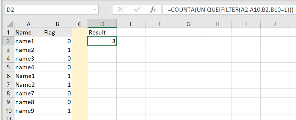
New Answer 9/28/2022

Now you can use FILTER function to achieve it:

=COUNTA(UNIQUE(FILTER(A2:A10,B2:B10=1)))

Mong