How to find probability distribution and parameters for real data? (Python 3)

Question

I have a dataset from sklearn and I plotted the distribution of the load_diabetes.target data (i.e. the values of the regression that the load_diabetes.data are used to predict).

I used this because it has the fewest number of variables/attributes of the regression sklearn.datasets.

Using Python 3, How can I get the distribution-type and parameters of the distribution this most closely resembles?

All I know the target values are all positive and skewed (positve skew/right skew). . . Is there a way in Python to provide a few distributions and then get the best fit for the target data/vector? OR, to actually suggest a fit based on the data that's given? That would be realllllly useful for people who have theoretical statistical knowledge but little experience with applying it to "real data".

Bonus Would it make sense to use this type of approach to figure out what your posterior distribution would be with "real data" ? If no, why not?

from sklearn.datasets import load_diabetes
import matplotlib.pyplot as plt
import seaborn as sns; sns.set()
import pandas as pd

#Get Data
data = load_diabetes()
X, y_ = data.data, data.target

#Organize Data
SR_y = pd.Series(y_, name="y_ (Target Vector Distribution)")

#Plot Data
fig, ax = plt.subplots()
sns.distplot(SR_y, bins=25, color="g", ax=ax)
plt.show()

Philippa

You could throw a couple of fits against the data and then go with the one that yields the smallest fitting error. – Backspace

Is the kde curve in your plot the function you want? – Labyrinthine

@Philip; for that, would you take the distributions from here: docs.scipy.org/doc/scipy/reference/stats.html ? Kind of picking and choosing which ones may fit the best? How do you test the fit if you dont know the parameters of the sample distribution? – Philippa

@ZichenWang not necessarily. Ultimately, I would be looking for one of these distributions: pymc-devs.github.io/pymc3/api.html with specific parameters and a fit error – Philippa

This answer shows all the scipy.stats distributions available, perhaps you can combine a few of these to generate your desired distribution. – Kynan

Answer 1

To the best of my knowledge, there is no automatic way of obtaining the distribution type and parameters of a sample (as inferring the distribution of a sample is a statistical problem by itself).

In my opinion, the best you can do is:

(for each attribute)

• Try to fit each attribute to a reasonably large list of possible distributions (e.g. see Fitting empirical distribution to theoretical ones with Scipy (Python)? for an example with Scipy)

• Evaluate all your fits and pick the best one. This can be done by performing a Kolmogorov-Smirnov test between your sample and each of the distributions of the fit (you have an implementation in Scipy, again), and picking the one that minimises D, the test statistic (a.k.a. the difference between the sample and the fit).

Bonus: It would make sense - as you'll be building a model on each of the variables as you pick a fit for each one - although the goodness of your prediction would depend on the quality of your data and the distributions you are using for fitting. You are building a model, after all.

Swiss

Look here if you need to view all the scipy.stats distributions. – Kynan

But how to differentiate between single-modal and multimodal distribution? E.g., here (imgur.com/a/NZKxxRv) I could see 3 modes of normal distribution or just a single one, if to be bold enough. – Boondocks

This article outlines how to use the Fitter library to automatically identify which of scipy's distributions best fit the data towardsdatascience.com/… – Wolford

Answer 2

Use this approach

import scipy.stats as st
def get_best_distribution(data):
    dist_names = ["norm", "exponweib", "weibull_max", "weibull_min", "pareto", "genextreme"]
    dist_results = []
    params = {}
    for dist_name in dist_names:
        dist = getattr(st, dist_name)
        param = dist.fit(data)

        params[dist_name] = param
        # Applying the Kolmogorov-Smirnov test
        D, p = st.kstest(data, dist_name, args=param)
        print("p value for "+dist_name+" = "+str(p))
        dist_results.append((dist_name, p))

    # select the best fitted distribution
    best_dist, best_p = (max(dist_results, key=lambda item: item[1]))
    # store the name of the best fit and its p value

    print("Best fitting distribution: "+str(best_dist))
    print("Best p value: "+ str(best_p))
    print("Parameters for the best fit: "+ str(params[best_dist]))

    return best_dist, best_p, params[best_dist]

Oxysalt

Could you please explain this approach ? – Ecker

It is a complete version of the code in the answer above. They created a list of items for all of the possible distributions that could fit the data. Then they create a hypothesis using the p-score to determine how close that distribution matches the data. What ever has the highest p-score is considered the most accurate. That's because the higher p-score means the hypothesis is closest to reality. – Javelin

Is there a way for this code to also try truncated normal distributions? I added "truncnorm" to the list for my dataset, but the function always returns p value = 0. Thank you! – Molten

In this approach you are looking for max P as the best one. Shouldn't it be the min(p) to be selected? – Doubleheader

Hi , thanks for this approach. After getting the parameters of the distribution , how can I generate synthetic data from the same distribution ? Any idea ? – Suppurate

@Suppurate wouldn't you just sample from the distribution? – Inapprehensive

@Suppurate You should use: new_data = np.random.normal(params[0], params[1], number_of_samples). Here param[0 is mean and param[1] is stddev or sigma. – Hypogenous

Note for anonymous user, for my case, this function indicated a exponweib distribution. But later, realised that it was due to 2 wrong samples inside about 2000 samples. After correcting, the function output normal distribution. – Hypogenous

Answer 3

You can use that code to fit (according to the maximum likelihood) different distributions with your datas:

import matplotlib.pyplot as plt
import scipy
import scipy.stats

dist_names = ['gamma', 'beta', 'rayleigh', 'norm', 'pareto']

for dist_name in dist_names:
    dist = getattr(scipy.stats, dist_name)
    param = dist.fit(y)
    # here's the parameters of your distribution, scale, location

You can see a sample snippet about how to use the parameters obtained here: Fitting empirical distribution to theoretical ones with Scipy (Python)?

Then, you can pick the distribution with the best log likelihood (there are also other criteria to match the "best" distribution, such as Bayesian posterior probability, AIC, BIC or BICc values, ...).

For your bonus question, there's I think no generic answer. If your set of data is significant and obtained under the same conditions as the real word datas, you can do it.

Vitiligo

I implemented the above code and param displayed just 3 values. Should'nt they be equal to 5? – Publus

Additionally, The Expectation-Maximization (EM) algorithm is used instead of Conventional maximum likelihood estimation (MLE) in cases when dataset is not full - when some unobserved or hidden variables are present (they are referred to as latent variables) – Coquina

Answer 4

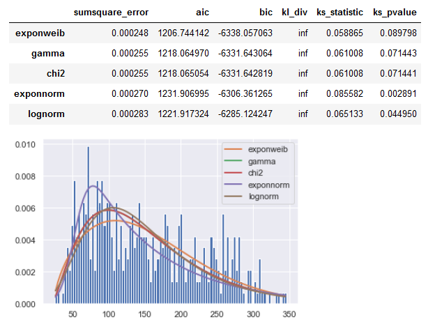
fitter provides an iteration process over possible fitting distributions.
It also outputs a plot and summary table with statistic values.

fitter package provides a simple class to identify the distribution from which a data samples is generated from. It uses 80 distributions from Scipy and allows you to plot the results to check what is the most probable distribution and the best parameters.

So basically the same iterative fit test procedure as described in other answers, but conveniently executed by the module.

Result for your SR_y series:

Code:

from sklearn.datasets import load_diabetes
from fitter import Fitter, get_common_distributions

#Get Data - from question
data = load_diabetes()
X, y_ = data.data, data.target
#Organize Data - from question
SR_y = pd.Series(y_, name="y_ (Target Vector Distribution)")


# fitter
distributions_set = get_common_distributions()
distributions_set.extend(['arcsine', 'cosine', 'expon', 'weibull_max', 'weibull_min', 
                          'dweibull', 't', 'pareto', 'exponnorm', 'lognorm',
                         "norm", "exponweib", "weibull_max", "weibull_min", "pareto", "genextreme"])  

f = Fitter(SR_y, distributions = distributions_set) 
f.fit()
f.summary()

Parameters of those fitted distributions as a dict:

f.fitted_param

{'expon': (25.0, 127.13348416289594),
 'cauchy': (132.95536663886972, 52.62243313109789),
 'gamma': (2.496376511103246, 20.737715299081657, 52.63462302106953),
 'norm': (152.13348416289594, 77.00574586945044),
 'chi2': (4.9927545799818525, 20.737731375230684, 26.317289176495912),
 'rayleigh': (14.700761411215545, 111.3948791009951),
 'uniform': (25.0, 321.0),
 'powerlaw': (1.0864390359784966, -6.82376066691087, 352.82376073752073),
 'cosine': (159.01669793410446, 65.6033963343604),
 'arcsine': (-6.99037533558757, 352.9903753355876),
 'exponpow': (0.15440493125261756, 24.999999999999996, 16.00571403929016),
 'weibull_max': (0.168196678837625, 346.0000000000001, 1.6686318895897978),
 'weibull_min': (0.2750237375428041, 24.999999999999996, 6.998090013988461),
 'dweibull': (1.6343449438402855, 157.0247145542748, 73.64165822064473),
 'pareto': (0.6022461735477798, -0.06169932009129858, 25.06169863339018),
 'exponnorm': (6.298770105099791, 53.6065309642624, 15.642251691931591),
 't': (127967.50529392948, 152.12481045573628, 76.98521783304597),
 'exponweib': (0.9662752277542657, 1.6900600238468133, 24.142487003378918, 150.25955880342326),
 'lognorm': (0.44469088248930166, -29.00650970868123, 164.71283014005542),
 'genextreme': (0.029317901766728702, 116.52312667345038, 63.454691756821106)}

---

To get a list of all available distributions:

from fitter import get_distributions

get_distributions()

Testing for all of them takes a long time, so it's best to use the implemened get_common_distributions() and potentially extend them with likely distribution as done in the code above.

---

Make sure to have the current (1.4.1 or newer) fitter version installed:

import fitter

print(fitter.version)

I had logging errors with a previous one and for my conda environment I needed:

conda install -c bioconda fitter

Kob

The Fitter Library is really cool. Thanks! – Intermit

Answer 5

This code also works:

import pandas as pd
import numpy as np
import scipy
from scipy import stats

#Please write below the name of the statistical distributions that you would like to check.
#Full list is here: https://docs.scipy.org/doc/scipy/reference/stats.html
dist_names = ['weibull_min','norm','weibull_max','beta',
              'invgauss','uniform','gamma','expon',   
              'lognorm','pearson3','triang']

#Read your data and set y_std to the column that you want to fit.
y_std=pd.read_csv('my_df.csv')
y_std=y_std['column_A']

#-------------------------------------------------
chi_square_statistics = []
size=len(y_std)

# 20 equi-distant bins of observed Data 
percentile_bins = np.linspace(0,100,20)
percentile_cutoffs = np.percentile(y_std, percentile_bins)
observed_frequency, bins = (np.histogram(y_std, bins=percentile_cutoffs))
cum_observed_frequency = np.cumsum(observed_frequency)

# Loop through candidate distributions
for distribution in dist_names:
    # Set up distribution and get fitted distribution parameters
    dist = getattr(scipy.stats, distribution)
    param = dist.fit(y_std)
    print("{}\n{}\n".format(dist, param))

    # Get expected counts in percentile bins
    # cdf of fitted sistrinution across bins
    cdf_fitted = dist.cdf(percentile_cutoffs, *param)
    expected_frequency = []
    for bin in range(len(percentile_bins)-1):
        expected_cdf_area = cdf_fitted[bin+1] - cdf_fitted[bin]
        expected_frequency.append(expected_cdf_area)

    # Chi-square Statistics
    expected_frequency = np.array(expected_frequency) * size
    cum_expected_frequency = np.cumsum(expected_frequency)
    ss = sum (((cum_expected_frequency - cum_observed_frequency) ** 2) / cum_observed_frequency)
    chi_square_statistics.append(ss)


#Sort by minimum ch-square statistics
results = pd.DataFrame()
results['Distribution'] = dist_names
results['chi_square'] = chi_square_statistics
results.sort_values(['chi_square'], inplace=True)


print ('\nDistributions listed by goodness of fit:')
print ('............................................')
print (results)

Lantana

Answer 6

On a similar question (see here) you may be interrested in @Michel_Baudin answer explaining. His code assesses around 40 different distributions available OpenTURNS library and chooses the best one according to the BIC criterion. Looks something like that:

import openturns as ot

sample = ot.Sample([[x] for x in your_data_list])
tested_factories = ot.DistributionFactory.GetContinuousUniVariateFactories()
best_model, best_bic = ot.FittingTest.BestModelBIC(sample, tested_factories)

Phylogeny