How to SUM duration in Google Sheets?

Question

Time started time end      Duration
6:02:53 PM   6:11:07 PM    0:08:13
6:11:22 PM   6:20:33 PM    0:09:11
6:20:48 PM   6:32:21 PM    0:11:34
6:32:44 PM   6:39:04 PM    0:06:20
6:39:28 PM   7:00:41 PM    0:21:13
7:01:00 PM   7:09:16 PM    0:08:16
7:09:40 PM   7:16:03 PM    0:06:23
7:16:03 PM   7:24:21 PM    0:08:17
7:24:45 PM   7:30:57 PM    0:06:12
7:31:27 PM   7:37:21 PM    0:05:54
7:37:21 PM   7:44:06 PM    0:06:45

I want sum of all duration entries in x hours x minutes x seconds like i have more then 1000 rows of duration when i try to use =SUM(C2:C100) I am not getting sum of total duration after sum of 24:00:00 24 hours it starts from 00:00:00

for example sum of total duration gets 24:00:00 between range of c1:c8 it will start from 00:00:00 from c9: next range kindly assist me how to overcome this issue

Helsie

Answer 1

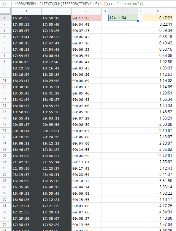
try:

=ARRAYFORMULA(TEXT(SUM(IFERROR(TIMEVALUE(C:C))), "[h]:mm:ss"))

spreadsheet demo

Tessie

Answer 2

Wherever you put the =SUM(), Select that cell and do Format>Number>More Formats>Custom Number formatting, and put the same formatting that Player0 put in his answer:

Kantar

not working it shows the same i have given my copy of duration please help – Helsie

Doesn't work for me shows 00:00:00 – Raffinate

@Helsie This formula works on your sheet =SUMPRODUCT(B:B-A:A+(A:A>B:B)) – Kantar

@Helsie : I have added a new answer (that I got to work), hope it may help: https://mcmap.net/q/332053/-how-to-sum-duration-in-google-sheets – Nador

Answer 3

What worked for me to resolve a similar problem was a suggestion by user ttarchala in Google Sheets Query multi condition sum of time duration.

I used N() function as he said, and my final formula for the duration is:

=IF(To<>"", N(To-From+(To<From))*24, "")

with To and From being Named ranges for End Time and Start Time respectively.

N() function converts the time delta into a number. Multiplied by 24, this gives the hours in decimal format, such as 2 hours 30 minutes = 2.5 hours.

From there on, there is no problem with using the built-in Sum function to calculate the total duration as a decimal. Such as, the total duration of 27 hrs 10 minutes is shown as 27.16. This sufficed for my purposes.

Time delta is calculated using a formula from https://webapps.stackexchange.com/questions/104829/calculate-time-difference-between-times-past-midnight to take into account past-midnight differences.

And the first condition, To<>"", makes sure the formula is not showing in empty cells. As soon as the End Time is filled into "To" column, the decimal duration is calculated. Then it can be used in the regular Sum function.

This seemed shorter and easier than the formulas suggested above so I am sharing it in the hopes it may help someone else. Using thus formula, I just added up the Sum of time I spent looking for this solution: 3.34 hours :)

Suricate

Answer 4

It's a formatting problem. You formatted your reply as HH:MM:SS, therefore the number displayed is not showing the date, which would have been incremented by one. If you multiply your sum by 24, and then format the result as a pure number, you will get a number that goes above 24, and will show you the number of hours, and its decimals. If you use those hours in further calculations, the result will be correct.

Shortridge

Answer 5

In cell C1, use the formula

=IF((B1-A1)>=0, B1-A1, 1+B1-A1)

Explanation: the problem is durations that exceed the 24 hour limit, as you say.

Google Sheets has become a bit deceptive here, as it will show the correct duration for the individual time interval, but if you SUM over it, it will actually deduct the value!

A       B       C
23:39   1:10    1:31

When you SUM then Google Sheets will see the value in cell C1 as if it was the beginning of the same day as the time in A1. So when you in C1 do =B1-A1 then it will register as a negative duration! But it won't show up as that!

In C1 use this formula, =IF((B1-A1)>=0, B1-A1, 1+B1-A1) for individual cells in column C, when you see that cells in column B has exceeded the 24-hour limit once. The duration in C1 should still show 1:31, but now the result when doing SUM over a range of cells in column C, like =SUM(C1:C2), will now show the correct and strictly additive sum. You can safely copy this formula to all cells in column C.

PS: cells in all of the columns can have Automatic or no formatting (which I think defaults to Automatic), if your time inputs look like the above. So you don't need to format all of those cells to Time or Duration. BUT remember to format the SUM cell to Format -> Number -> Duration.

PPS: if you are manually inputting the times (for for instance time tracking), then the easiest way to keep the much simpler =B1-A1 formula is to split the time up into two rows, like this:

A       B       C
23:39   0:00    0:21
0:00    1:10    1:10

Then the SUM of cells in column C still becomes 1:31.

Nador