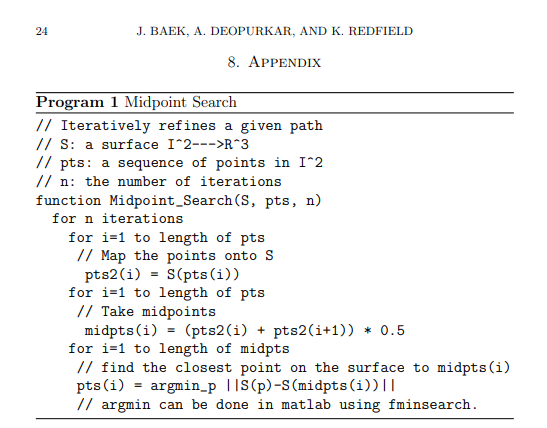
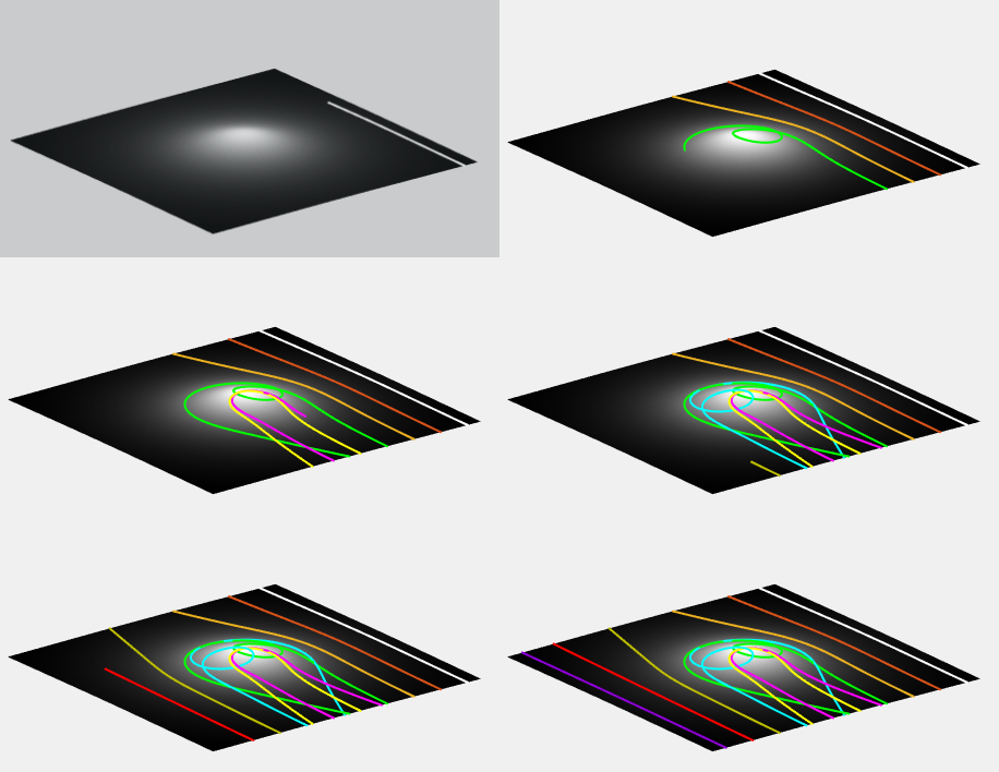
Using the midpoint search method:
![enter image description here]()
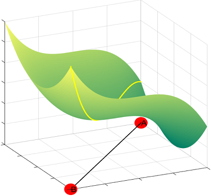
applied to the function f(x,y) = x^3 + y^2, I am projecting the points of the line segment on the XY plane y = x from x = -1 to x = 1.
To get an idea, with one iteration and only 4 points on the line on the XY plane, the black spheres are these 4 original points of the line projected on the surface, while the red dots are the midpoints in a single iteration, and the yellow dots the result of the projection of the red dots along the normal to the surface:
![enter image description here]()
Using Matlab fmincon() and after 5 iterations we can get a geodesic from point A to point B:
![enter image description here]()
Here is the code:
% Creating the surface
x = linspace(-1,1);
y = linspace(-1,1);
[x,y] = meshgrid(x,y);
z = x.^3 + y.^2;
S = [x;y;z];
h = surf(x,y,z)
set(h,'edgecolor','none')
colormap summer

% Number of points
n = 1000;

% Line to project on the surface with n values to get a feel for it...
t = linspace(-1,1,n);
height = t.^3 + t.^2;
P = [t;t;height];

% Plotting the projection of the line on the surface:
hold on
%plot3(P(1,:),P(2,:),P(3,:),'o')

for j=1:5
% First midpoint iteration updates P...
P = [P(:,1), (P(:,1:end-1) + P(:,2:end))/2, P(:,end)];
%plot3(P(1,:), P(2,:), P(3,:), '.', 'MarkerSize', 20)

A = zeros(3,size(P,2));
for i = 1:size(P,2)
% Starting point will be the vertical projection of the mid-points:
    A(:,i) = [P(1,i), P(2,i), P(1,i)^3 + P(2,i)^2];
end

% Linear constraints:
nonlincon = @nlcon;

% Placing fmincon in a loop for all the points

for i = 1:(size(A,2))
    % Objective function:
    objective = @(x)(P(1,i) - x(1))^2 + (P(2,i) - x(2))^2 + (P(3,i)-x(3))^2;
    A(:,i) = fmincon(objective, A(:,i), [], [], [], [], [], [], nonlincon);
end

P = A;
end

plot3(P(1,:), P(2,:), P(3,:), '.', 'MarkerSize', 5,'Color','y')
In a separate file with name nlcon.m:
function[c,ceq] = nlcon(x)
   c   = [];
   ceq = x(3) - x(1)^3 - x(2)^2;
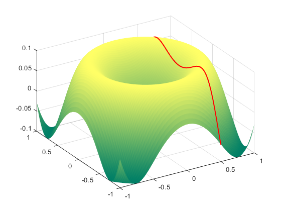
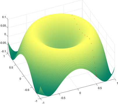
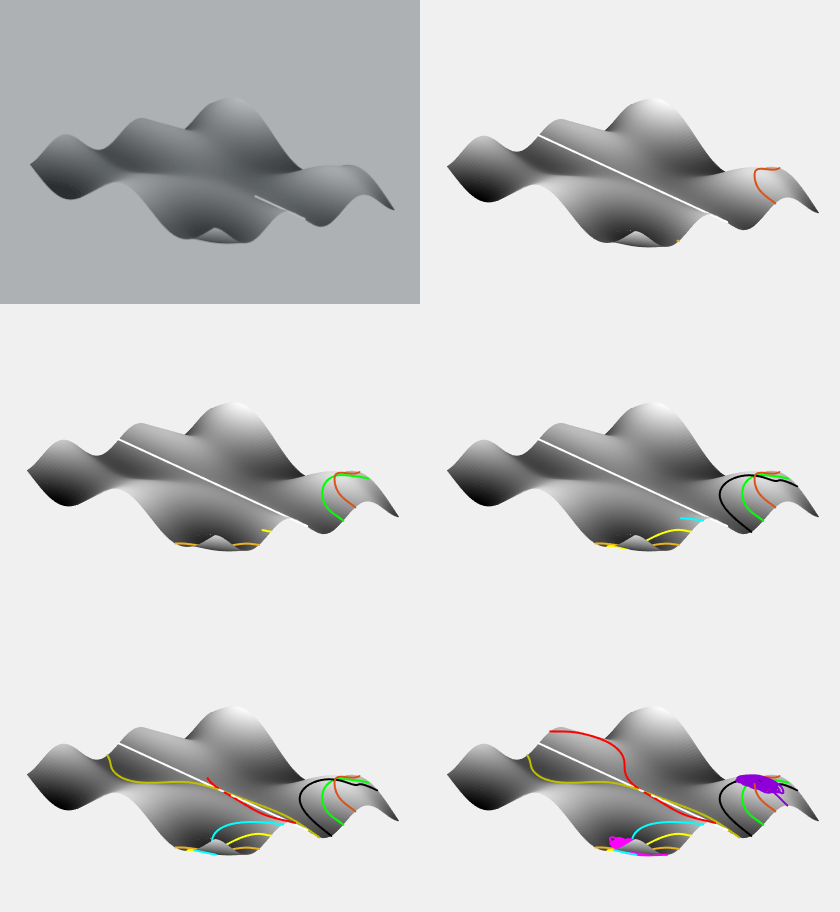
Same for a geodesic on a really cool surface with a straight, non-diagonal line on XY:
![enter image description here]()
% Creating the surface
x = linspace(-1,1);
y = linspace(-1,1);
[x,y] = meshgrid(x,y);
z = sin(3*(x.^2+y.^2))/10;
S = [x;y;z];
h = surf(x,y,z)
set(h,'edgecolor','none')
colormap summer

% Number of points
n = 1000;

% Line to project on the surface with n values to get a feel for it...
t = linspace(-1,1,n);
height = sin(3*((.5*ones(1,n)).^2+ t.^2))/10;
P = [(.5*ones(1,n));t;height];

% Plotting the line on the surface:
hold on
%plot3(P(1,:),P(2,:),P(3,:),'o')

for j=1:2
% First midpoint iteration updates P...
P = [P(:,1), (P(:,1:end-1) + P(:,2:end))/2, P(:,end)];
%plot3(P(1,:), P(2,:), P(3,:), '.', 'MarkerSize', 20)

A = zeros(3,size(P,2));
for i = 1:size(P,2)
% Starting point will be the vertical projection of the first mid-point:
    A(:,i) = [P(1,i), P(2,i), sin(3*(P(1,i)^2+ P(2,i)^2))/10];
end

% Linear constraints:
nonlincon = @nonlincon;

% Placing fmincon in a loop for all the points

for i = 1:(size(A,2))
    % Objective function:
    objective = @(x)(P(1,i) - x(1))^2 + (P(2,i) - x(2))^2 + (P(3,i)-x(3))^2;
    A(:,i) = fmincon(objective, A(:,i), [], [], [], [], [], [], nonlincon);
end

P = A;
end

plot3(P(1,:), P(2,:), P(3,:), '.', 'MarkerSize',5,'Color','r')
with the nonlinear constraint in nonlincon.m:
function[c,ceq] = nlcon(x)
   c   = [];
   ceq = x(3) - sin(3*(x(1)^2+ x(2)^2))/10;
One nagging concern is the possibility of overfitting to the curve with this method, and this latter plot is an example of it. So I adjusted the code to just select one beginning and one ending point, and allowing the iterative process to find the rest of the curve, which for 100 iterations seemed to be heading in the right direction:
![enter image description here]()
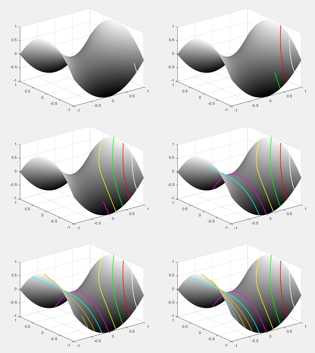
The above examples seem to follow a linear projection on the XY plane, but fortunately this is not a fixed pattern, which would cast further doubt on the method. See for instance the hyperbolic paraboloid x^2 - y^2:
![enter image description here]()
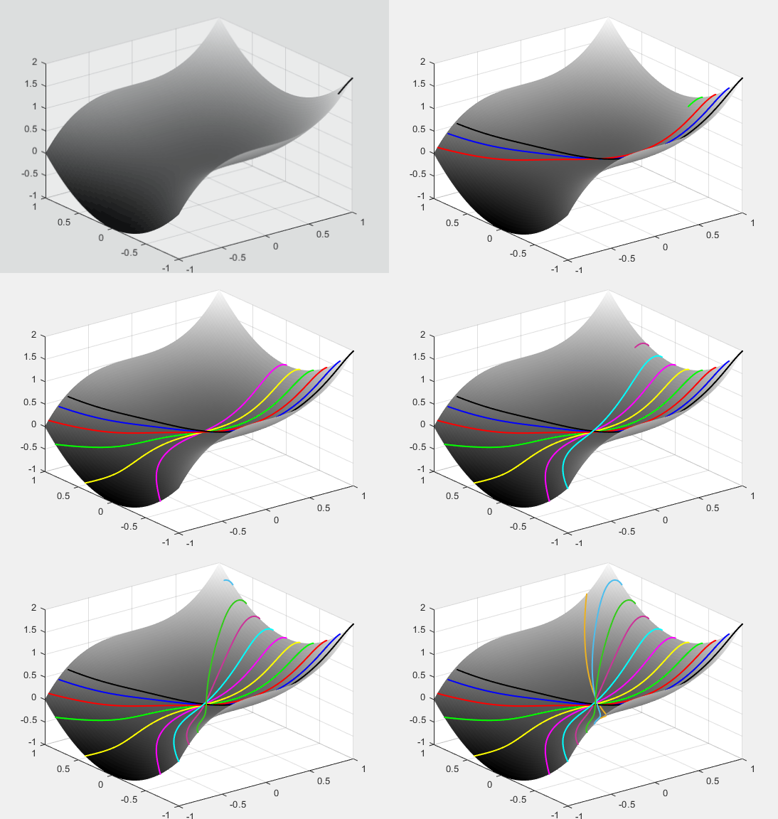
Notice that there are algorithms to advance or push geodesic lines along a surface f(x,y) with small increments determined by the starting points and the normal vector to the surface, as in here. Thanks to the work of Alvise Vianello looking into the JS in that simulation and his sharing in GitHub, I was able to turn that algorithm into Matlab code, generating this plot for the first example, f(x,y) = x^3 + y^2:
![enter image description here]()
Here is the Matlab code:
x = linspace(-1,1);
y = linspace(-1,1);
[x,y] = meshgrid(x,y);
z = x.^3 + y.^2;
S = [x;y;z];
h = surf(x,y,z)
set(h,'edgecolor','none')
colormap('gray');
hold on

f = @(x,y) x.^3 + y.^2; % The actual surface

dfdx = @(x,y) (f(x + eps, y) - f(x - eps, y))/(2 * eps); % ~ partial f wrt x
dfdy = @(x,y) (f(x, y + eps) - f(x, y - eps))/(2 * eps); % ~ partial f wrt y

N = @(x,y) [- dfdx(x,y), - dfdy(x,y), 1]; % Normal vec to surface @ any pt.

C = {'k','b','r','g','y','m','c',[.8 .2 .6],[.2,.8,.1],[0.3010 0.7450 0.9330],[0.9290 0.6940 0.1250],[0.8500 0.3250 0.0980]}; % Color scheme

for s = 1:11     % No. of lines to be plotted.
start = -5:5;    % Distributing the starting points of the lines.
y0 = start(s)/5; % Fitting the starting pts between -1 and 1 along y axis.
x0 = 1;          % Along x axis always starts at 1.
dx0 = 0;         % Initial differential increment along x
dy0 = 0.05;      % Initial differential increment along y
step_size = 0.000008; % Will determine the progression rate from pt to pt.
eta =  step_size / sqrt(dx0^2 + dy0^2); % Normalization.
eps = 0.0001;          % Epsilon
max_num_iter = 100000; % Number of dots in each line.

x = [[x0, x0 + eta * dx0], zeros(1,max_num_iter - 2)]; % Vec of x values
y = [[y0, y0 + eta * dy0], zeros(1,max_num_iter - 2)]; % Vec of y values

for i = 2:(max_num_iter - 1)  % Creating the geodesic:
            xt = x(i);        % Values at point t of x, y and the function:
            yt = y(i);
            ft = f(xt,yt);

            xtm1 = x(i - 1);  % Values at t minus 1 (prior point) for x,y,f
            ytm1 = y(i - 1);
            ftm1 = f(xtm1,ytm1);

            xsymp = xt + (xt - xtm1); % Adding the prior difference forward:
            ysymp = yt + (yt - ytm1);
            fsymp = ft + (ft - ftm1);

            df = fsymp - f(xsymp,ysymp); % Is the surface changing? How much?
            n = N(xt,yt);                % Normal vector at point t
            gamma = df * n(3);           % Scalar x change f x z value of N

            xtp1 = xsymp - gamma * n(1); % Gamma to modulate incre. x & y.
            ytp1 = ysymp - gamma * n(2);

            x(i + 1) = xtp1;
            y(i + 1) = ytp1;
end

P = [x; y; f(x,y)]; % Compiling results into a matrix.

indices = find(abs(P(1,:)) < 1); % Avoiding lines overshooting surface.
P = P(:,indices);
indices = find(abs(P(2,:)) < 1);
P = P(:,indices);

    units = 15; % Deternines speed (smaller, faster)
    packet = floor(size(P,2)/units);
    P = P(:,1: packet * units);

  for k = 1:packet:(packet * units)
        hold on
        plot3(P(1, k:(k+packet-1)), P(2,(k:(k+packet-1))), P(3,(k:(k+packet-1))),...
            '.', 'MarkerSize', 3.5,'color',C{s})
        drawnow
  end

end
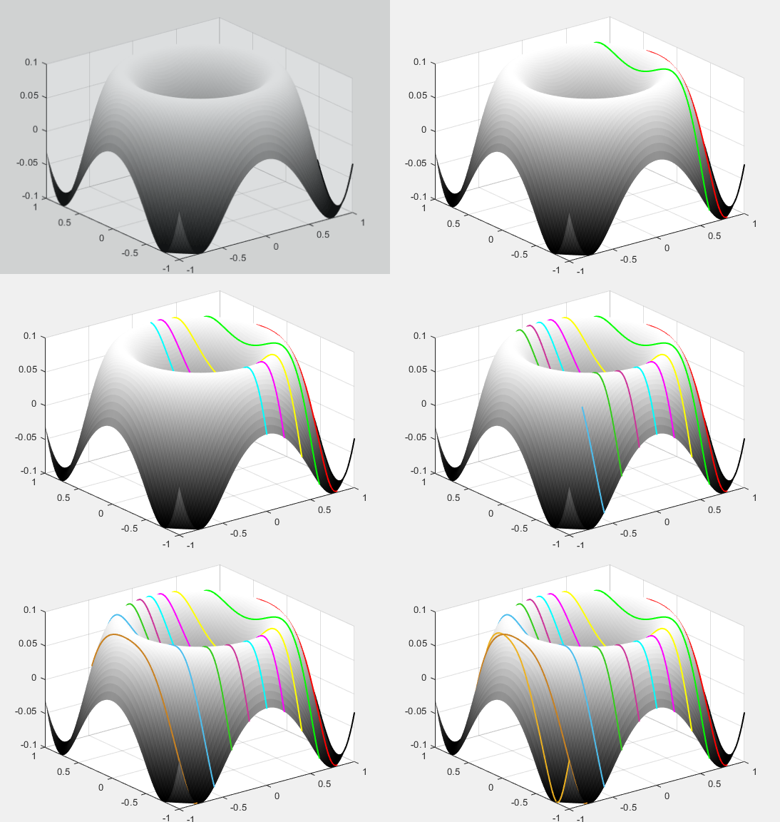
And here is an earlier example from above, but now calculated differently, and with lines starting side by side, following geodesics (no point-to-point trajectory):
![enter image description here]()
    x = linspace(-1,1);
    y = linspace(-1,1);
    [x,y] = meshgrid(x,y);
    z = sin(3*(x.^2+y.^2))/10;
    S = [x;y;z];
    h = surf(x,y,z)
    set(h,'edgecolor','none')
    colormap('gray');
    hold on

    f = @(x,y) sin(3*(x.^2+y.^2))/10; % The actual surface

    dfdx = @(x,y) (f(x + eps, y) - f(x - eps, y))/(2 * eps); % ~ partial f wrt x
    dfdy = @(x,y) (f(x, y + eps) - f(x, y - eps))/(2 * eps); % ~ partial f wrt y

    N = @(x,y) [- dfdx(x,y), - dfdy(x,y), 1]; % Normal vec to surface @ any pt.

    C = {'k','r','g','y','m','c',[.8 .2 .6],[.2,.8,.1],[0.3010 0.7450 0.9330],[0.7890 0.5040 0.1250],[0.9290 0.6940 0.1250],[0.8500 0.3250 0.0980]}; % Color scheme

    for s = 1:11     % No. of lines to be plotted.
    start = -5:5;    % Distributing the starting points of the lines.
    x0 = -start(s)/5; % Fitting the starting pts between -1 and 1 along y axis.
    y0 = -1;          % Along x axis always starts at 1.
    dx0 = 0;         % Initial differential increment along x
    dy0 = 0.05;      % Initial differential increment along y
    step_size = 0.00005; % Will determine the progression rate from pt to pt.
    eta =  step_size / sqrt(dx0^2 + dy0^2); % Normalization.
    eps = 0.0001;          % Epsilon
    max_num_iter = 100000; % Number of dots in each line.

    x = [[x0, x0 + eta * dx0], zeros(1,max_num_iter - 2)]; % Vec of x values
    y = [[y0, y0 + eta * dy0], zeros(1,max_num_iter - 2)]; % Vec of y values

    for i = 2:(max_num_iter - 1)  % Creating the geodesic:
                xt = x(i);        % Values at point t of x, y and the function:
                yt = y(i);
                ft = f(xt,yt);

                xtm1 = x(i - 1);  % Values at t minus 1 (prior point) for x,y,f
                ytm1 = y(i - 1);
                ftm1 = f(xtm1,ytm1);

                xsymp = xt + (xt - xtm1); % Adding the prior difference forward:
                ysymp = yt + (yt - ytm1);
                fsymp = ft + (ft - ftm1);

                df = fsymp - f(xsymp,ysymp); % Is the surface changing? How much?
                n = N(xt,yt);                % Normal vector at point t
                gamma = df * n(3);           % Scalar x change f x z value of N

                xtp1 = xsymp - gamma * n(1); % Gamma to modulate incre. x & y.
                ytp1 = ysymp - gamma * n(2);

                x(i + 1) = xtp1;
                y(i + 1) = ytp1;
    end

    P = [x; y; f(x,y)]; % Compiling results into a matrix.

    indices = find(abs(P(1,:)) < 1); % Avoiding lines overshooting surface.
    P = P(:,indices);
    indices = find(abs(P(2,:)) < 1);
    P = P(:,indices);
    units = 35; % Deternines speed (smaller, faster)
    packet = floor(size(P,2)/units);
    P = P(:,1: packet * units);


  for k = 1:packet:(packet * units)
        hold on

        plot3(P(1, k:(k+packet-1)), P(2,(k:(k+packet-1))), P(3,(k:(k+packet-1))), '.', 'MarkerSize', 5,'color',C{s})
        drawnow
  end

    end
Some more examples:
![enter image description here]()
    x = linspace(-1,1);
    y = linspace(-1,1);
    [x,y] = meshgrid(x,y);
    z = x.^2 - y.^2;
    S = [x;y;z];
    h = surf(x,y,z)
    set(h,'edgecolor','none')
    colormap('gray');


    f = @(x,y) x.^2 - y.^2; % The actual surface

    dfdx = @(x,y) (f(x + eps, y) - f(x - eps, y))/(2 * eps); % ~ partial f wrt x
    dfdy = @(x,y) (f(x, y + eps) - f(x, y - eps))/(2 * eps); % ~ partial f wrt y

    N = @(x,y) [- dfdx(x,y), - dfdy(x,y), 1]; % Normal vec to surface @ any pt.

    C = {'b','w','r','g','y','m','c',[0.75, 0.75, 0],[0.9290, 0.6940, 0.1250],[0.3010 0.7450 0.9330],[0.1290 0.6940 0.1250],[0.8500 0.3250 0.0980]}; % Color scheme

    for s = 1:11     % No. of lines to be plotted.
    start = -5:5;    % Distributing the starting points of the lines.
    x0 = -start(s)/5; % Fitting the starting pts between -1 and 1 along y axis.
    y0 = -1;          % Along x axis always starts at 1.
    dx0 = 0;         % Initial differential increment along x
    dy0 = 0.05;      % Initial differential increment along y
    step_size = 0.00005; % Will determine the progression rate from pt to pt.
    eta =  step_size / sqrt(dx0^2 + dy0^2); % Normalization.
    eps = 0.0001;          % Epsilon
    max_num_iter = 100000; % Number of dots in each line.

    x = [[x0, x0 + eta * dx0], zeros(1,max_num_iter - 2)]; % Vec of x values
    y = [[y0, y0 + eta * dy0], zeros(1,max_num_iter - 2)]; % Vec of y values

    for i = 2:(max_num_iter - 1)  % Creating the geodesic:
                xt = x(i);        % Values at point t of x, y and the function:
                yt = y(i);
                ft = f(xt,yt);

                xtm1 = x(i - 1);  % Values at t minus 1 (prior point) for x,y,f
                ytm1 = y(i - 1);
                ftm1 = f(xtm1,ytm1);

                xsymp = xt + (xt - xtm1); % Adding the prior difference forward:
                ysymp = yt + (yt - ytm1);
                fsymp = ft + (ft - ftm1);

                df = fsymp - f(xsymp,ysymp); % Is the surface changing? How much?
                n = N(xt,yt);                % Normal vector at point t
                gamma = df * n(3);           % Scalar x change f x z value of N

                xtp1 = xsymp - gamma * n(1); % Gamma to modulate incre. x & y.
                ytp1 = ysymp - gamma * n(2);

                x(i + 1) = xtp1;
                y(i + 1) = ytp1;
    end

    P = [x; y; f(x,y)]; % Compiling results into a matrix.

    indices = find(abs(P(1,:)) < 1); % Avoiding lines overshooting surface.
    P = P(:,indices);
    indices = find(abs(P(2,:)) < 1);
    P = P(:,indices);
    units = 45; % Deternines speed (smaller, faster)
    packet = floor(size(P,2)/units);
    P = P(:,1: packet * units);

  for k = 1:packet:(packet * units)
        hold on
        plot3(P(1, k:(k+packet-1)), P(2,(k:(k+packet-1))), P(3,(k:(k+packet-1))), '.', 'MarkerSize', 5,'color',C{s})
        drawnow
  end

  end
Or this one:
![enter image description here]()
    x = linspace(-1,1);
    y = linspace(-1,1);
    [x,y] = meshgrid(x,y);
    z = .07 * (.1 + x.^2 + y.^2).^(-1);
    S = [x;y;z];
    h = surf(x,y,z)
    zlim([0 8])
    set(h,'edgecolor','none')
    colormap('gray');
    axis off
    hold on

    f = @(x,y) .07 * (.1 + x.^2 + y.^2).^(-1);    % The actual surface

    dfdx = @(x,y) (f(x + eps, y) - f(x - eps, y))/(2 * eps); % ~ partial f wrt x
    dfdy = @(x,y) (f(x, y + eps) - f(x, y - eps))/(2 * eps); % ~ partial f wrt y

    N = @(x,y) [- dfdx(x,y), - dfdy(x,y), 1]; % Normal vec to surface @ any pt.

     C = {'w',[0.8500, 0.3250, 0.0980],[0.9290, 0.6940, 0.1250],'g','y','m','c',[0.75, 0.75, 0],'r',...
         [0.56,0,0.85],'m'}; % Color scheme

    for s = 1:10     % No. of lines to be plotted.
    start = -9:2:9;
    x0 = -start(s)/10;
    y0 = -1;          % Along x axis always starts at 1.
    dx0 = 0;         % Initial differential increment along x
    dy0 = 0.05;      % Initial differential increment along y
    step_size = 0.00005; % Will determine the progression rate from pt to pt.
    eta =  step_size / sqrt(dx0^2 + dy0^2); % Normalization.
    eps = 0.0001;          % EpsilonA
    max_num_iter = 500000; % Number of dots in each line.

    x = [[x0, x0 + eta * dx0], zeros(1,max_num_iter - 2)]; % Vec of x values
    y = [[y0, y0 + eta * dy0], zeros(1,max_num_iter - 2)]; % Vec of y values

    for i = 2:(max_num_iter - 1)  % Creating the geodesic:
                xt = x(i);        % Values at point t of x, y and the function:
                yt = y(i);
                ft = f(xt,yt);

                xtm1 = x(i - 1);  % Values at t minus 1 (prior point) for x,y,f
                ytm1 = y(i - 1);
                ftm1 = f(xtm1,ytm1);

                xsymp = xt + (xt - xtm1); % Adding the prior difference forward:
                ysymp = yt + (yt - ytm1);
                fsymp = ft + (ft - ftm1);

                df = fsymp - f(xsymp,ysymp); % Is the surface changing? How much?
                n = N(xt,yt);                % Normal vector at point t
                gamma = df * n(3);           % Scalar x change f x z value of N

                xtp1 = xsymp - gamma * n(1); % Gamma to modulate incre. x & y.
                ytp1 = ysymp - gamma * n(2);

                x(i + 1) = xtp1;
                y(i + 1) = ytp1;
    end

     P = [x; y; f(x,y)]; % Compiling results into a matrix.

    indices = find(abs(P(1,:)) < 1.5); % Avoiding lines overshooting surface.
    P = P(:,indices);
    indices = find(abs(P(2,:)) < 1);
    P = P(:,indices);

    units = 15; % Deternines speed (smaller, faster)
    packet = floor(size(P,2)/units);
    P = P(:,1: packet * units);

  for k = 1:packet:(packet * units)
        hold on
        plot3(P(1, k:(k+packet-1)), P(2,(k:(k+packet-1))), P(3,(k:(k+packet-1))),...
            '.', 'MarkerSize', 3.5,'color',C{s})
        drawnow
  end

    end
Or a sinc function:
![enter image description here]()
    x = linspace(-10, 10);
    y = linspace(-10, 10);
    [x,y] = meshgrid(x,y);
    z = sin(1.3*sqrt (x.^ 2 + y.^ 2) + eps)./ (sqrt (x.^ 2 + y.^ 2) + eps);
    S = [x;y;z];
    h = surf(x,y,z)
    set(h,'edgecolor','none')
    colormap('gray');
    axis off
    hold on

    f = @(x,y) sin(1.3*sqrt (x.^ 2 + y.^ 2) + eps)./ (sqrt (x.^ 2 + y.^ 2) + eps);   % The actual surface

    dfdx = @(x,y) (f(x + eps, y) - f(x - eps, y))/(2 * eps); % ~ partial f wrt x
    dfdy = @(x,y) (f(x, y + eps) - f(x, y - eps))/(2 * eps); % ~ partial f wrt y

    N = @(x,y) [- dfdx(x,y), - dfdy(x,y), 1]; % Normal vec to surface @ any pt.

    C = {'w',[0.8500, 0.3250, 0.0980],[0.9290, 0.6940, 0.1250],'g','y','r','c','m','w',...
         [0.56,0,0.85],[0.8500, 0.7250, 0.0980],[0.2290, 0.1940, 0.6250],'w',...
         [0.890, 0.1940, 0.4250],'y',[0.2290, 0.9940, 0.3250],'w',[0.1500, 0.7250, 0.0980],...
         [0.8500, 0.3250, 0.0980],'m','w'}; % Color scheme

    for s = 1:12     % No. of lines to be plotted.

    x0 = 10;
    y0 = 10;          % Along x axis always starts at 1.
    dx0 = -0.001*(cos(pi /2 *s/11));         % Initial differential increment along x
    dy0 = -0.001*(sin(pi /2 *s/11));         % Initial differential increment along y
    step_size = 0.0005; % Will determine the progression rate from pt to pt.
    % Making it smaller increases the length of the curve.
    eta =  step_size / sqrt(dx0^2 + dy0^2); % Normalization.
    eps = 0.0001;          % EpsilonA
    max_num_iter = 500000; % Number of dots in each line.

    x = [[x0, x0 + eta * dx0], zeros(1,max_num_iter - 2)]; % Vec of x values
    y = [[y0, y0 + eta * dy0], zeros(1,max_num_iter - 2)]; % Vec of y values

    for i = 2:(max_num_iter - 1)  % Creating the geodesic:
                xt = x(i);        % Values at point t of x, y and the function:
                yt = y(i);
                ft = f(xt,yt);

                xtm1 = x(i - 1);  % Values at t minus 1 (prior point) for x,y,f
                ytm1 = y(i - 1);
                ftm1 = f(xtm1,ytm1);

                xsymp = xt + (xt - xtm1); % Adding the prior difference forward:
                ysymp = yt + (yt - ytm1);
                fsymp = ft + (ft - ftm1);

                df = fsymp - f(xsymp,ysymp); % Is the surface changing? How much?
                n = N(xt,yt);                % Normal vector at point t
                gamma = df * n(3);           % Scalar x change f x z value of N

                xtp1 = xsymp - gamma * n(1); % Gamma to modulate incre. x & y.
                ytp1 = ysymp - gamma * n(2);

                x(i + 1) = xtp1;
                y(i + 1) = ytp1;
    end

     P = [x; y; f(x,y)]; % Compiling results into a matrix.

    indices = find(abs(P(1,:)) < 10); % Avoiding lines overshooting surface.
    P = P(:,indices);
    indices = find(abs(P(2,:)) < 10);
    P = P(:,indices);

    units = 15; % Deternines speed (smaller, faster)
    packet = floor(size(P,2)/units);
    P = P(:,1: packet * units);

  for k = 1:packet:(packet * units)
        hold on
        plot3(P(1, k:(k+packet-1)), P(2,(k:(k+packet-1))), P(3,(k:(k+packet-1))),...
            '.', 'MarkerSize', 3.5,'color',C{s})
        drawnow
  end

    end
And one very last one:
![enter image description here]()
    x = linspace(-1.5,1.5);
    y = linspace(-1,1);
    [x,y] = meshgrid(x,y);
    z = 0.5 *y.*sin(5 * x) - 0.5 * x.*cos(5 * y)+1.5;
    S = [x;y;z];
    h = surf(x,y,z)
    zlim([0 8])
    set(h,'edgecolor','none')
    colormap('gray');
    axis off
    hold on

    f = @(x,y) 0.5 *y.* sin(5 * x) - 0.5 * x.*cos(5 * y)+1.5;     % The actual surface

    dfdx = @(x,y) (f(x + eps, y) - f(x - eps, y))/(2 * eps); % ~ partial f wrt x
    dfdy = @(x,y) (f(x, y + eps) - f(x, y - eps))/(2 * eps); % ~ partial f wrt y

    N = @(x,y) [- dfdx(x,y), - dfdy(x,y), 1]; % Normal vec to surface @ any pt.

     C = {'w',[0.8500, 0.3250, 0.0980],[0.9290, 0.6940, 0.1250],'g','y','k','c',[0.75, 0.75, 0],'r',...
         [0.56,0,0.85],'m'}; % Color scheme

    for s = 1:11     % No. of lines to be plotted.
    start = [0, 0.7835,  -0.7835, 0.5877, -0.5877, 0.3918, -0.3918, 0.1959, -0.1959, 0.9794, -0.9794];
    x0 = start(s);
    y0 = -1;          % Along x axis always starts at 1.
    dx0 = 0;         % Initial differential increment along x
    dy0 = 0.05;      % Initial differential increment along y
    step_size = 0.00005; % Will determine the progression rate from pt to pt.
    % Making it smaller increases the length of the curve.
    eta =  step_size / sqrt(dx0^2 + dy0^2); % Normalization.
    eps = 0.0001;          % EpsilonA
    max_num_iter = 500000; % Number of dots in each line.

    x = [[x0, x0 + eta * dx0], zeros(1,max_num_iter - 2)]; % Vec of x values
    y = [[y0, y0 + eta * dy0], zeros(1,max_num_iter - 2)]; % Vec of y values

    for i = 2:(max_num_iter - 1)  % Creating the geodesic:
                xt = x(i);        % Values at point t of x, y and the function:
                yt = y(i);
                ft = f(xt,yt);

                xtm1 = x(i - 1);  % Values at t minus 1 (prior point) for x,y,f
                ytm1 = y(i - 1);
                ftm1 = f(xtm1,ytm1);

                xsymp = xt + (xt - xtm1); % Adding the prior difference forward:
                ysymp = yt + (yt - ytm1);
                fsymp = ft + (ft - ftm1);

                df = fsymp - f(xsymp,ysymp); % Is the surface changing? How much?
                n = N(xt,yt);                % Normal vector at point t
                gamma = df * n(3);           % Scalar x change f x z value of N

                xtp1 = xsymp - gamma * n(1); % Gamma to modulate incre. x & y.
                ytp1 = ysymp - gamma * n(2);

                x(i + 1) = xtp1;
                y(i + 1) = ytp1;
    end

     P = [x; y; f(x,y)]; % Compiling results into a matrix.

    indices = find(abs(P(1,:)) < 1.5); % Avoiding lines overshooting surface.
    P = P(:,indices);
    indices = find(abs(P(2,:)) < 1);
    P = P(:,indices);

    units = 15; % Deternines speed (smaller, faster)
    packet = floor(size(P,2)/units);
    P = P(:,1: packet * units);

  for k = 1:packet:(packet * units)
        hold on
        plot3(P(1, k:(k+packet-1)), P(2,(k:(k+packet-1))), P(3,(k:(k+packet-1))),...
            '.', 'MarkerSize', 3.5,'color',C{s})
        drawnow
  end

    end
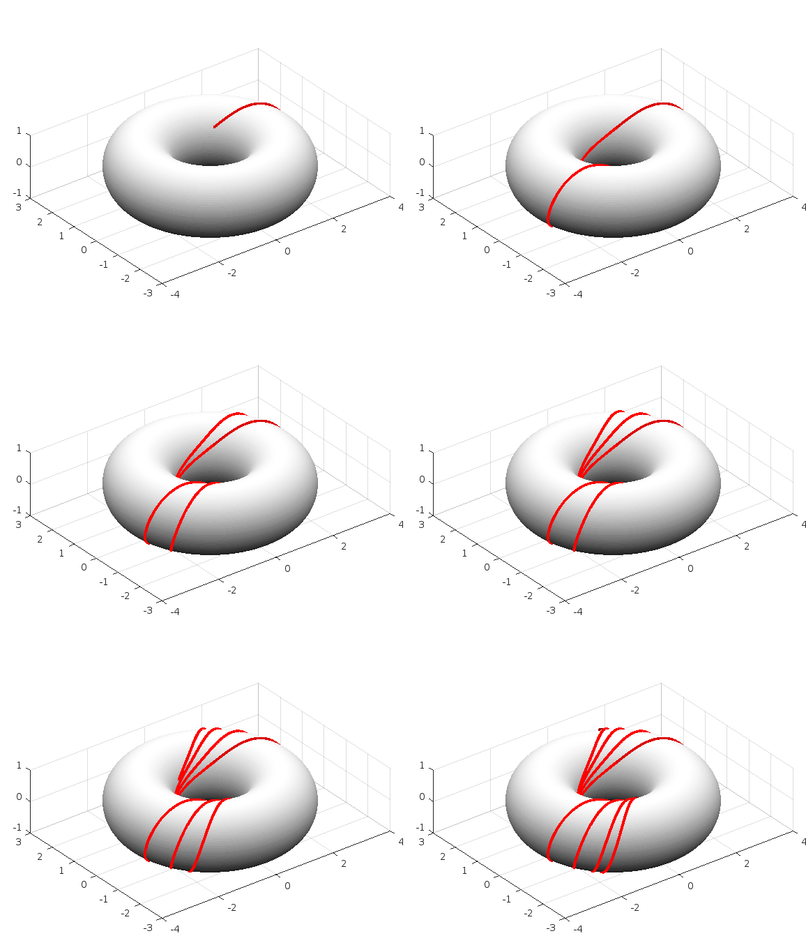
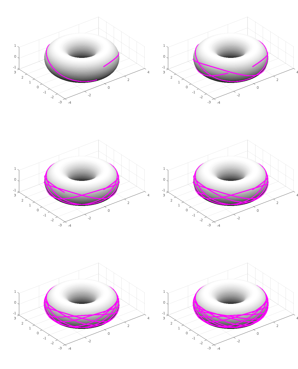
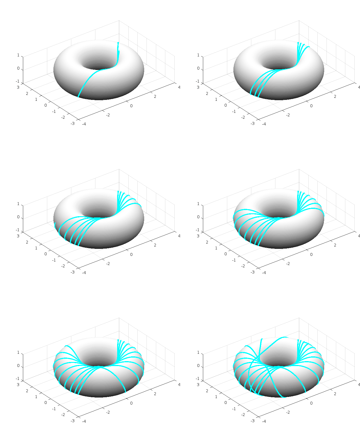
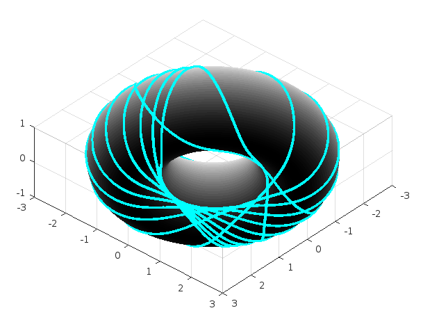
On a torus this becomes more complicated, and so far I haven't been able to adapt this code to it. As a reference, the code provided by Paul Chesler in here does provide with an option. It involves saving a file tor.m as
function xp=tor(t,x)
xp=zeros(4,1);
xp(1)=x(2);
xp(2)=-(2+cos(x(1)))*sin(x(1))*x(4)^2;
xp(3)=x(4);
xp(4)=2*(sin(x(1))/(2+cos(x(1))))*x(2)*x(4);
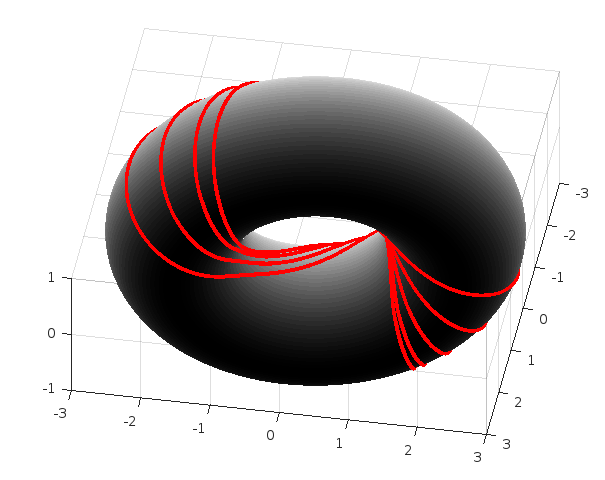
and in another file torus.m plot the torus and call the function above to solve a system of second order differential equations. Here it is for different geodesics:
![enter image description here]()
from below:
![enter image description here]()
with torus.m:
[u,v]=meshgrid(linspace(0,2*pi,100),linspace(0,2*pi,100));
x=(2+cos(u)).*cos(v);
y=(2+cos(u)).*sin(v);
z=sin(u);

h=surf(x,y,z);
set(h,'edgecolor','none');
colormap('gray');
daspect([1 1 1])

tspan = linspace(pi,100*pi,1000000);
[t,X]=ode45('tor',tspan ,[pi,.1,-pi/2,.2]);
u=X(:,1);
v=X(:,3);
x=(2+cos(u)).*cos(v);
y=(2+cos(u)).*sin(v);
z=sin(u);

P=[x y z];
disp(size(P))

units = 10; % Deternines speed (smaller, faster)
packet = floor(size(P,1)/units);

  for k = 1:packet:(packet * units)
        hold on
        plot3(P(k:(k+packet-1),1), P((k:(k+packet-1)),2), P((k:(k+packet-1)),3),...
            '.-', 'MarkerSize', 3.5,'color','r', 'LineWidth', 3)
        drawnow
        pause(2)
  end
or
![enter image description here]()
[u,v]=meshgrid(linspace(0,2*pi,100),linspace(0,2*pi,100));
x=(2+cos(u)).*cos(v);
y=(2+cos(u)).*sin(v);
z=sin(u);

h=surf(x,y,z);
set(h,'edgecolor','none');
colormap('gray');
daspect([1 1 1])

tspan = linspace(pi,100*pi,1000000);
[t,X]=ode45('tor',tspan ,[pi/6,.1,-pi/2,.2]);
u=X(:,1);
v=X(:,3);
x=(2+cos(u)).*cos(v);
y=(2+cos(u)).*sin(v);
z=sin(u);

P=[x y z];
disp(size(P))

units = 10; % Deternines speed (smaller, faster)
packet = floor(size(P,1)/units);

  for k = 1:packet:(packet * units)
        hold on
        plot3(P(k:(k+packet-1),1), P((k:(k+packet-1)),2), P((k:(k+packet-1)),3),...
            '.-', 'MarkerSize', 3.5,'color','m', 'LineWidth', 3)
        drawnow
        pause(2)
  end
or
![enter image description here]()
from below:
![enter image description here]()
tspan = linspace(pi,100*pi,1000000); defines the limits of integration along 1e^6 pts, and [3/4 * pi,.1,-pi/2,.2], the parametric values for a starting point (on the last example).
On a sphere:
![enter image description here]()
code here.


