Can fit curve with scipy minimize but not with scipy curve_fit

Question

I am trying to fit the functiony= 1-a(1-bx)**n to some experimental data using scipy curve_fit. The model only exists for y>0, so I clip the calculated values to enforce this. The code is shown below

import numpy as np
import scipy.optimize
import matplotlib.pyplot as plt

# Driver function for scipy.minimize

def driver_func(x, xobs, yobs):

    # Evaluate the fit function with the current parameter estimates

    ynew = myfunc(xobs, *x)
    yerr = np.sum((ynew - yobs) ** 2)

    return yerr

# Define function

def myfunc(x, a, b, n):

    y = 1.0 - a * np.power(1.0 - b * x, n) 
    y = np.clip(y, 0.00, None )

    return y

if __name__ == "__main__":

    # Initialise data

    yobs = np.array([0.005, 0.000, 0.000, 0.000, 0.000, 0.000, 0.000, 0.004, 
                    0.048, 0.119, 0.199, 0.277, 0.346, 0.395, 0.444, 0.469, 
                    0.502, 0.527, 0.553, 0.582, 0.595, 0.603, 0.612, 0.599])
    xobs = np.array([0.013, 0.088, 0.159, 0.230, 0.292, 0.362, 0.419, 0.471,
                    0.528, 0.585, 0.639, 0.687, 0.726, 0.772, 0.814, 0.854,
                    0.889, 0.924, 0.958, 0.989, 1.015, 1.045, 1.076, 1.078])

    # Initial guess

    p0 = [2.0, 0.5, 2.0]

    # Check fit pre-regression

    yold = myfunc(xobs, *p0)
    plt.plot(xobs, yobs, 'ko', label='data', fillstyle='none')
    plt.plot(xobs, yold, 'g-', label='pre-fit: a=%4.2f, b=%4.2f, n=%4.2f' % tuple(p0))

    # Fit curve using SCIPY CURVE_FIT

    try:
        popt, pcov = scipy.optimize.curve_fit(myfunc, xobs, yobs, p0=p0)
    except:
        print("Could not fit data using SCIPY curve_fit")
    else:
        ynew = myfunc(xobs, *popt)
        plt.plot(xobs, ynew, 'r-', label='post-curve_fit: a=%4.2f, b=%4.2f, n=%4.2f' % tuple(popt))

    # Fit curve using SCIPY MINIMIZE

    res = scipy.optimize.minimize(driver_func, p0, args=(xobs, yobs), method='Nelder-Mead')
    ynw2 = myfunc(xobs, *res.x)
    plt.plot(xobs, ynw2, 'y-', label='post-minimize: a=%4.2f, b=%4.2f, n=%4.2f' % tuple(res.x))

    plt.legend()
    plt.show()

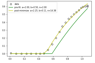
I also used SCIPY MINIMIZE to achieve the same thing. As the image below shows, MINIMIZE works, but CURVE_FIT basically runs out of evalautions and gives up, even though the starting guess is not that far away from the MINIMIZE solution (at least visually). Would appreciate any thoughts on why curve_fit seems not to be working here.

Thanks!

Update: Following the comments by mikuszefski I made the following adjustments 1. removed the clipping from the fit function as follows:

def myfunc_noclip(x, a, b, n):
    y = 1.0 - a * np.power(1.0 - b * x, n) 
    return y

2. introduced clipped arrays by removing data below a threshold

   ymin = 0.01
   xclp = xobs[np.where(yobs >= ymin)]
   yclp = yobs[np.where(yobs >= ymin)]
   

3. improved the initial guess (again visually)

   p0 = [1.75, 0.5, 2.0]
   

4. updated the call to curve_fit

   popt, pcov = scipy.optimize.curve_fit(myfunc_noclip, xclp, yclp, p0=p0)
   

But this does not seem to have helped as the following plot shows:

Other posts on stackoverflow seem to suggest that scipy curve_fit has trouble fitting curves where one of the fit parameters is an exponent eg SciPy curve_fit not working when one of the parameters to fit is a power so I am guessing that I have the same problem. Not sure how to solve it though ...

Dinahdinan

Answer 1

This problem is caused by the clipping in the function definition. The two minimization methods work fundamentally different and, therefore, react very differently to this clipping. Here minimize is used with Nelder-Mead, which is a gradient free method. The algorithm, hence is not calculating numerical gradients and not estimating any Jacobians. In contrasts the least-squares, which is eventually called by curve_fit, does exactly this. However, approximating a gradient and from this any Jacobian is somewhat questionable if the function is not continuous. As mentioned before, this discontinuity is introduced by the np.clip. When removed, one can easily see, that the P0 guess is not as good as it seems with clipping included. The curve_fit does converge with increased maxfev=5000, though, while the minimize immediately fails when changing the method to method='CG'. To see the algorithms difficulties one may try to provide manually the jac.

Some notes: 1) Concerning the clipping it might be a good idea to remove data that is clipped, such the according problem is avoided. 2) Looking at the covariance matrix the error of n and the correlation with the other values is extremely high.

So here is what I get from

import numpy as np
import scipy.optimize
import matplotlib.pyplot as plt

# Driver function for scipy.minimize
def driver_func( x, xobs, yobs ):
    # Evaluate the fit function with the current parameter estimates
    ynew = myfunc( xobs, *x)
    yerr = np.sum( ( ynew - yobs ) ** 2 )
    return yerr

# Define functions
def myfunc( x, a, b, n ):
    y = 1.0 - a * np.power( 1.0 - b * x, n ) 
    y = np.clip( y, 0.00, None )
    return y

def myfunc_noclip( x, a, b, n ):
    y = 1.0 - a * np.power( 1.0 - b * x, n ) 
    return y

if __name__ == "__main__":

    # Initialise data
    yobs = np.array([
        0.005, 0.000, 0.000, 0.000, 0.000, 0.000, 0.000, 0.004, 
        0.048, 0.119, 0.199, 0.277, 0.346, 0.395, 0.444, 0.469, 
        0.502, 0.527, 0.553, 0.582, 0.595, 0.603, 0.612, 0.599
    ])
    xobs = np.array([
        0.013, 0.088, 0.159, 0.230, 0.292, 0.362, 0.419, 0.471,
        0.528, 0.585, 0.639, 0.687, 0.726, 0.772, 0.814, 0.854,
        0.889, 0.924, 0.958, 0.989, 1.015, 1.045, 1.076, 1.078
    ])

    # Clipped data
    ymin = 0.01
    xclp = xobs[ np.where( yobs >= ymin ) ]
    yclp = yobs[ np.where( yobs >= ymin ) ]

    # Initial guess
    p0 = [ 2.0, 0.5, 2.0 ]

    # Check fit pre-regression
    yold = myfunc( xobs, *p0 )
    plt.plot( xobs, yobs, 'ko', label='data', fillstyle='none' )
    plt.plot( xobs, yold, 'g-', label='pre-fit: a=%4.2f, b=%4.2f, n=%4.2f' % tuple( p0 ) )

    # Fit curve using SCIPY CURVE_FIT
    try:
        popt, pcov = scipy.optimize.curve_fit( myfunc, xobs, yobs, p0=p0, maxfev=5000 )
    except:
        print("Could not fit data using SCIPY curve_fit")
    else:
        ynew = myfunc( xobs, *popt )
        plt.plot( xobs, ynew, 'r-', label="curve-fit: a=%4.2f, b=%4.2e, n=%4.2f" % tuple( popt ) )

    # Fit curve using SCIPY CURVE_FIT on clipped data
    p0 = [ 1.75, 1e-4, 1e3 ]
    try:
        popt, pcov = scipy.optimize.curve_fit( myfunc_noclip, xclp, yclp, p0=p0 )
    except:
        print("Could not fit data using SCIPY curve_fit")
    else:
        ynew = myfunc_noclip( xobs, *popt )
        plt.plot( xobs, ynew, 'k-', label="curve-fit clipped data: a=%4.2f, b=%4.2e, n=%4.2f" % tuple( popt ) )

    # Fit curve using SCIPY MINIMIZE
    p0 = [ 2.0, 0.5, 2.0 ]
    res = scipy.optimize.minimize( driver_func, p0, args=( xobs, yobs ), method='Nelder-Mead' )
    # ~res = scipy.optimize.minimize(driver_func, p0, args=(xobs, yobs), method='CG')
    ynw2 = myfunc( xobs, *res.x )
    plt.plot( xobs, ynw2, 'y--', label='Nelder-Mead 1: a=%4.2f, b=%4.2f, n=%4.2f' % tuple( res.x ) )
    p0 = [ 2.4, 3.6e-4, 5.6e3 ]
    res = scipy.optimize.minimize( driver_func, p0, args=( xobs, yobs ), method='Nelder-Mead' )
    # ~res = scipy.optimize.minimize(driver_func, p0, args=(xobs, yobs), method='CG')
    ynw2 = myfunc( xobs, *res.x )
    plt.plot( xobs, ynw2, 'b:', label='Nelder-Mead 2: a=%4.2f, b=%4.2e, n=%4.2e' % tuple( res.x ) )

    plt.legend( loc=2 )
    plt.ylim( -0.05, 0.7 )
    plt.grid()
    plt.show()

So I'd say it works okeyish. I get an overflow warning, though.

Emelinaemeline

Hi mikuszefski thanks for your comments. I have updated the post to include the results of the changes that you suggested in (1) but unfortunately they did not help. Not sure how to address (2) - the equation is generic and seems to work OK on other datasets so I guess I was just unlucky with the data in the example. I have the same problem with other sets of (x,y) data – Dinahdinan

@Dinahdinan Made and according edit. Works fine here. – Emelinaemeline

Hi @Emelinaemeline - thanks for taking the time to investigate this further. I ran your version of the code and it works fine but if I comment out the statement p0 = [ 1.75, 1e-4, 1e3 ] then it doesn't. It is possible to estimate the initial parameters using other properties of the data and these starting values are (unfortunately) non-physical. So the problem seems to be my data and model rather than curvefit – Dinahdinan

@Dinahdinan I think the problem is the extremely high correlation of the parameters in this model. The chi^2 minimum is probably very very stretched in some diagonal manner in parameter space. As a consequence some minor variation in data might lead major changes in fit results. In this sense it is a model problem, yes. You see that the initial slope is related to b * n so you can shift between them easily. Depending on the physics behind the problem, you might try a different saturation model. – Emelinaemeline