Change phase of a signal in frequency domain (MatLab)

Question

I posted this question on dsp.stackexchange, and was informed that it was more relevant for stackoverflow as it is primarily a programming question:

I am attempting to write a code which allows me to change the phase of a signal in the frequency domain. However, my output isn't exactly correct, so something must be wrong. For a simple example assume that we have the function y = sin(2*pi*t) and want to implement a phase shift of -pi/2. My code looks as follows:

clear all
close all

N = 64; %number of samples
fs = 10; %sampling frequency
ts = 1/fs; %sample interval
tmax = (N-1)*ts;
t = 0:ts:tmax;
y = sin(2*pi*t);

figure
plot(t,y)

% We do the FT
f = -fs/2:fs/(N-1):fs/2;
Y = fftshift(fft(y));

% Magnitude spectrum
figure
plot(f,abs(Y));

phase = angle(Y);

% Phase spectrum
figure
plot(f,phase)

Y = ifftshift(Y)

% Attempt at phase shift
Y = Y.*exp(-i*2*pi*f*pi/2);

% Inverse FT
u = ifft(Y);

figure
plot(t,real(u))

All plots look OK except for the final plot which looks as follows:

This looks almost correct but not quite. If anyone can give me some pointers as to how my code can be corrected in order to fix this, I would greatly appreciate it! I have a feeling my mistake has something to do with the line Y = Y.*exp(-i*2*pi*f*pi/2);, but I'm not sure how to fix it.

Okra

Answer 1

I can't really get into the Fourier analysis details (because I do not really know them), but I can offer a working solution with some hints:

First of all, You should express Your wave in imaginary terms, i.e.:

y = exp(1i*2*pi*t);

And what's even more crucial, You have to truly shift only the phase, without messing with the whole spectrum:

% Attempt at phase shift
Y = abs(Y).*exp(1i*angle(Y)-1i*pi/4); % -pi/4 shift

You should note that the shift isn't related to frequency anymore, which I guess makes sense. Finally You can plot the results:

figure
plot(t,real(u),'k')
hold on
plot(t,real(y),'r')

real(y) is actually a cosine function, and You started with sine, but hopefully You get the idea. For pi/4 shift i got something like this (started with red, finished with black):

Gipson

Answer 2

You made 3 major mistakes in your code design.

1. The input vector of a FFT is interpreted as a period of a signal with is repeated infinitely. This means your input vector should contain an integer number of complete periods of your sine signal. You have an input vector of 64 samples and a sample rate of 10. This results in 6.4 periods of your sine wave, which leads to leakage. If you inspect the frequency spectrum after performing the FFT, you will see, that there are not two clean frequency lines, but a lot of frequency components around two places.
2. After correcting your input vector, there should be only two single frequencies with values which are not close to zeros. 62 frequency components will consist of numerical noise very close to zero. Calculating the phase of these values results in garbage data.
3. A phase shift of pi/2 in time domain is equivalent by a shift in time domain by N/4 if N is the number of input samples.

I modified your code. You will find it below. With the variable M you can change the number of periods of a sine wave in your input vector. In the example I have set M=3.

clear all;
close all;

T = 1;  %length of sampling sequence in s
N = 64; %number of samples
M = 3; % number of periods per sequence
ts = T/N; %sample interval
fs = 1/ts %sampling frequency
tmax = (N-1)*ts;
t = 0:ts:tmax;
y = sin(2*pi*M*t);

fig01 = figure;
plot(t,y);
grid on;

%% We do the FT
Y = fft(y);

%% We create a frequency vector in natural order
% -fs/2, ..., 0, ... +fs/2
f =fftshift(( 0:(fs-1)) - fs/2);

%% Show Magnitude spectrum
% There shold be only two lines at -M and +M
figure;
plot(f,abs(Y),'o');
grid on;

%% Attempt at phase shift
% y/t) -> Y(w)
% y(t-t0) -> Y(w) * exp(-i*w*t0)
% Phase shift of pi/2 in frequncy domain is equavalent to as time shift
% of T/4 in time domain

Y = Y.*exp(-i*2*pi*f*T/4);

% Inverse FT
u = ifft(Y);

figure
hold on;
plot(t,real(u),'b-');
plot(t,real(y),'r-');
hold off;
grid;

Input signal with three periods of a sine signal

Spectrum of input signal. Frequency lines at -3 and +3

Input signal (blue) and phase shifted signal (red)

Bukharin

Answer 3

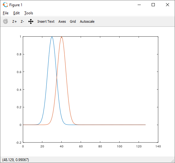
I just want to expand on Heinz’s code above. The code above introduces additional parameters to generate the test signal which is something that I have struggled with as well. After doing some in depth study I realized that these additional parameters are not needed and an explanation without them might make things clearer. The main simplification to keep in mind is this: the (Discrete) Fourier transform takes whatever number of points (elements of a data array) you give it and maps them to zero to 2 * pi. If N is the number of points, then you see 2 * pi / N throughout the calculations. The remainder of the explanation is in the Matlab code below.

function val = gauss(x, sigma, xc)
exponent = ((x-xc).^2)./(2*sigma);
val       = (exp(-exponent));
endfunction

% Shift a Signal in the Frequency Domain.
% Number of points in the signal:
N = 128;

% Create a sample point array.  It must be 0  to N-1 in steps of 1.
n=linspace(0,N-1,128);

% Generate a signal from the sample points.
g=gauss(n,20,30);

% The Fourier transform simply maps whatever number of points you give it
% to 0 to 2*pi.  It does not take into consideration signal sampling rate or any other
% external parameters.  Whatever set of points you give it, it maps them to the unit circle.
% Remember that a Fourier transform provides positive and negative frequency components centered
% about the zero frequency, called the DC offset.  For a  real signal the negative frequency components
% are the complex conjugate of the positive frequencies.  This is called conjugate symmetric.
% Generate the frequency index.
m = linspace(-N/2, (N/2 – 1), N);

% For N = 128, m will be -64 to 63.
% In the following 2*pi / N will appear everywhere and often that number will appear as a constant
% such as w = 2*pi / N.
% Let S be the number of data points to shift the signal.  Given the external parameters that were used
% to generate the signal you can back out what a point shift means, but the (Discrete) Fourier transform 
% doesn’t care.  It works on points, samples, or whatever you might call them.
S = 10;
% S = 10 means a 10 point shift.

% To introduce the shift in the frequency domain multiply the Fourier transform of the signal by
% exp(-i*(2*pi / N)*S* m) .  It might help to remember that exp(i*f) = cos(f) + i * sin(f) .
% Fourier transform the signal.
fg = fft(g);

% Shift the signal in the frequency domain.
fh = fg .* exp(-i*(2*pi / N)*S* m);

% Inverse transform to see the signal back in the special domain.  Note that we have to take the real
% part because even though the imaginary part will be very very small, the result will still be
% a complex number and it will confuse the graphing package.
h=real( ifft(fh) );

plot(n,g)
hold on
plot(n,h)

Fringe