How do you create a logit-normal distribution in Python?

Question

Following this post, I tried to create a logit-normal distribution by creating the LogitNormal class:

import numpy as np
import matplotlib.pyplot as plt
from scipy.special import logit
from scipy.stats import norm, rv_continuous


class LogitNormal(rv_continuous):
    def _pdf(self, x, **kwargs):
        return norm.pdf(logit(x), **kwargs)/(x*(1-x))


class OtherLogitNormal:
    def pdf(self, x, **kwargs):
        return norm.pdf(logit(x), **kwargs)/(x*(1-x))


fig, ax = plt.subplots()
values = np.linspace(10e-10, 1-10e-10, 1000)
sigma, mu = 1.78, 0
ax.plot(
    values, LogitNormal().pdf(values, loc=mu, scale=sigma), label='subclassed'
)
ax.plot(
    values, OtherLogitNormal().pdf(values, loc=mu, scale=sigma),
    label='not subclassed'
)
ax.legend()
fig.show()

However, the LogitNormal class does not produce the desired results. When I don't subclass rv_continuous it works. Why is that? I need the subclassing to work because I also need the other methods that come with it like rvs.

Btw, the only reason I am creating my own logit-normal distribution in Python is because the only implementations of that distribution that I could find were from the PyMC3 package and from the TensorFlow package, both of which are pretty heavy / overkill if you only need them for that one function. I already tried PyMC3, but apparently it doesn't do well with scipy I think, it always crashed for me. But that's a whole different story.

Propound

Why do you call LogitNormal().pdf? I guess you should call LogitNormal()._pdf. Cause _pdf is how you called the only method in LogitNormal class. – Aurita

Because re-defining _pdf or _cdf is how you subclass rv_continuous according to the documentation docs.scipy.org/doc/scipy/reference/generated/… and also the post that I linked in my question. – Propound

According to the source code rv_continuous.pdf method performs transformation of x values using loc and scale parameters. I guess you will get the same result with defaults: sigma, mu = 1, 0. – Aurita

I do. I'm confused. What does that mean? – Propound

Suppose the problem origins from doubled calculations. rv_continuous.pdf computes probability density function. And scipy.stats.norm.pdf computes probability density function. I guess that's all I can tell since I'm not familiar with these functions. Wish you luck. – Aurita

Answer 1

Forewords

I came across this problem this week and the only relevant issue I have found about it is this post. I have almost same requirement as the OP:

• Having a random variable for Logit Normal distribution.

But I also need:

• To be able to perform statistical test as well;
• While being compliant with the scipy random variable interface.

As @Jacques Gaudin pointed out the interface for rv_continous (see distribution architecture for details) does not ensure follow up for loc and scale parameters when inheriting from this class. And this is somehow misleading and unfortunate.

Implementing the __init__ method of course allow to create the missing binding but the trade off is: it breaks the pattern scipy is currently using to implement random variables (see an example of implementation for lognormal).

So, I took time to dig into the scipy code and I have created a MCVE for this distribution. Although it is not totally complete (it mainly misses moments overrides) it fits the bill for both OP and my purposes while having satisfying accuracy and performance.

MCVE

An interface compliant implementation of this random variable could be:

class logitnorm_gen(stats.rv_continuous):

    def _argcheck(self, m, s):
        return (s > 0.) & (m > -np.inf)
    
    def _pdf(self, x, m, s):
        return stats.norm(loc=m, scale=s).pdf(special.logit(x))/(x*(1-x))
    
    def _cdf(self, x, m, s):
        return stats.norm(loc=m, scale=s).cdf(special.logit(x))
    
    def _rvs(self, m, s, size=None, random_state=None):
        return special.expit(m + s*random_state.standard_normal(size))
    
    def fit(self, data, **kwargs):
        return stats.norm.fit(special.logit(data), **kwargs)

logitnorm = logitnorm_gen(a=0.0, b=1.0, name="logitnorm")

This implementation unlock most of the scipy random variables potential.

N = 1000
law = logitnorm(0.24, 1.31)             # Defining a RV
sample = law.rvs(size=N)                # Sampling from RV
params = logitnorm.fit(sample)          # Infer parameters w/ MLE
check = stats.kstest(sample, law.cdf)   # Hypothesis testing
bins = np.arange(0.0, 1.1, 0.1)         # Bin boundaries
expected = np.diff(law.cdf(bins))       # Expected bin counts

As it relies on scipy normal distribution we may assume underlying functions have the same accuracy and performance than normal random variable object. But it might indeed be subject to float arithmetic inaccuracy especially when dealing with highly skewed distributions at the support boundary.

Tests

To check out how it performs we draw some distribution of interest and check them. Let's create some fixtures:

def generate_fixtures(
    locs=[-2.0, -1.0, 0.0, 0.5, 1.0, 2.0],
    scales=[0.32, 0.56, 1.00, 1.78, 3.16],
    sizes=[100, 1000, 10000],
    seeds=[789, 123456, 999999]
):
    for (loc, scale, size, seed) in itertools.product(locs, scales, sizes, seeds):
        yield {"parameters": {"loc": loc, "scale": scale}, "size": size, "random_state": seed}

And perform checks on related distributions and samples:

eps = 1e-8
x = np.linspace(0. + eps, 1. - eps, 10000)

for fixture in generate_fixtures():
    
    # Reference:
    parameters = fixture.pop("parameters")
    normal = stats.norm(**parameters)
    sample = special.expit(normal.rvs(**fixture))
    
    # Logit Normal Law:
    law = logitnorm(m=parameters["loc"], s=parameters["scale"])
    check = law.rvs(**fixture)
    
    # Fit:
    p = logitnorm.fit(sample)
    trial = logitnorm(*p)
    resample = trial.rvs(**fixture)
    
    # Hypothetis Tests:
    ks = stats.kstest(check, trial.cdf)
    bins = np.histogram(resample)[1]
    obs = np.diff(trial.cdf(bins))*fixture["size"]
    ref = np.diff(law.cdf(bins))*fixture["size"]
    chi2 = stats.chisquare(obs, ref, ddof=2)

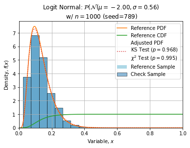
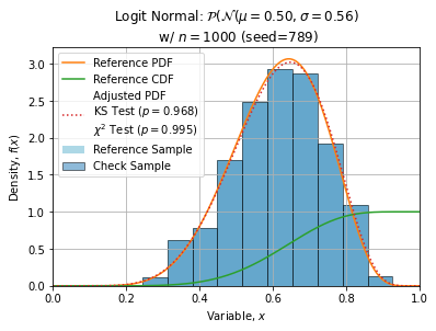
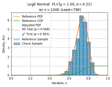
Some adjustments with n=1000, seed=789 (this sample is quite normal) are shown below:

Pass

Answer 2

If you look at the source code of the pdf method, you will notice that _pdf is called without the scale and loc keyword arguments.

   if np.any(cond):
        goodargs = argsreduce(cond, *((x,)+args+(scale,)))
        scale, goodargs = goodargs[-1], goodargs[:-1]
        place(output, cond, self._pdf(*goodargs) / scale)

It results that the kwargs in your overriding _pdf method is always an empty dictionary.

If you look a bit closer at the code, you will also notice that the scaling and location are handled by pdf as opposed to _pdf.

In your case, the _pdf method calls norm.pdf so the loc and scale parameters must somehow be available in LogitNormal._pdf.

You could for example pass scale and loc when creating an instance of LogitNormal and store the values as class attributes:

import numpy as np
import matplotlib.pyplot as plt
from scipy.special import logit
from scipy.stats import norm, rv_continuous


class LogitNormal(rv_continuous):
    def __init__(self, scale=1, loc=0):
        super().__init__(self)
        self.scale = scale
        self.loc = loc

    def _pdf(self, x):
        return norm.pdf(logit(x), loc=self.loc, scale=self.scale)/(x*(1-x))


fig, ax = plt.subplots()
values = np.linspace(10e-10, 1-10e-10, 1000)
sigma, mu = 1.78, 0
ax.plot(
    values, LogitNormal(scale=sigma, loc=mu).pdf(values), label='subclassed'
)
ax.legend()
fig.show()

Tributary

Thank you, this works! I know this is a different kind of question, but would you also happen to know what the inverse cdf / ppf looks like if implemented? Because, according to the documentation: "The default method _rvs relies on the inverse of the cdf, _ppf, applied to a uniform random variate. In order to generate random variates efficiently, either the default _ppf needs to be overwritten (e.g. if the inverse cdf can expressed in an explicit form) or a sampling method needs to be implemented in a custom _rvs method." – Propound

I don't know about the inverse cdf / pdf sorry, not very knowledgeable about statistics. Maybe asking on math.stackexchange.com would help? – Tributary

Ok, so here is a weird thing. I found out how to do it and wanted to edit your answer accordingly, but the interface won't let me, claming that the code is not formatted correctly. However, the alledged error is not in my edit, but in your quote. How can that be? If you literally open the edit and try to save it as it is, it won't work, unless you delete the quote. – Propound

Strange, maybe just post it as your answer. Nothing wrong in answering your question! – Tributary