How to fit a double Gaussian distribution in Python?

Question

I am trying to obtain a double Gaussian distribution for data (link) using Python. The raw data is of the form:

For the given data, I would like to obtain two Gaussian profiles for the peaks seen in figure. I tried it with the following code (source):

from sklearn import mixture
import matplotlib.pyplot
import matplotlib.mlab
import numpy as np
from pylab import *
data = np.genfromtxt('gaussian_fit.dat', skiprows = 1)
x = data[:, 0]
y = data[:, 1]
clf = mixture.GMM(n_components=2, covariance_type='full')
clf.fit((y, x))
m1, m2 = clf.means_
w1, w2 = clf.weights_
c1, c2 = clf.covars_
fig = plt.figure(figsize = (5, 5))
plt.subplot(111)
plotgauss1 = lambda x: plot(x,w1*matplotlib.mlab.normpdf(x,m1,np.sqrt(c1))[0], linewidth=3)
plotgauss2 = lambda x: plot(x,w2*matplotlib.mlab.normpdf(x,m2,np.sqrt(c2))[0], linewidth=3)
fig.savefig('gaussian_fit.pdf')

But I am not able to get the desired output. So, how can a double Gaussian distribution be obtained in Python?

Update

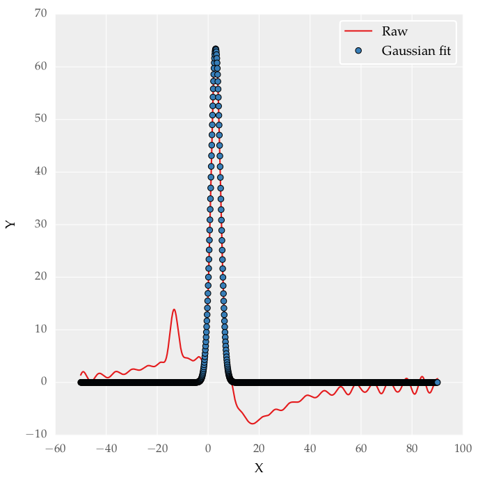
I was able to fit a single Gaussian distribution with the following code:

import pylab as plb
import matplotlib.pyplot as plt
from scipy.optimize import curve_fit
from scipy import asarray as ar,exp
import numpy as np

data = np.genfromtxt('gaussian_fit.dat', skiprows = 1)
x = data[:, 0]
y = data[:, 1]
n = len(x)
mean = sum(x*y)/n
sigma = sum(y*(x-mean)**2)/n


def gaus(x,a,x0,sigma):
    return a*exp(-(x-x0)**2/(2*sigma**2))


popt,pcov = curve_fit(gaus, x, y ,p0 = [1, mean, sigma])


fig = plt.figure(figsize = (5, 5))
plt.subplot(111)
plt.plot(x, y, label='Raw')
plt.plot(x, gaus(x, *popt), 'o', markersize = 4, label='Gaussian fit')
plt.xlabel('X')
plt.ylabel('Y')
plt.legend()
fig.savefig('gaussian_fit.pdf')

Bologna

as the answer by spfrnd suggests, you should first ask yourself why you want to fit Gaussians to the data, as PDFs are almost always defined to have a lower bound of 0 on their range (i.e. here you're considering fitting to 'negative' probability). you could transform the data by e.g. subtracting the minimum, and then GMMs might work better. You're likelier to get help fitting the GMMs if you show us the output and relevant data from your attempts. – Cone

Answer 1

You can't use scikit-learn for this, because the you are not dealing with a set of samples whose distribution you want to estimate. You could of course transform your curve to a PDF, sample it and then try to fit it using a Gaussian mixture model, but that seems to be a bit of an overkill to me.

Here's a solution using simple least square curve fitting. To get it to work I had to remove the background, i.e. ignore all data points with y < 5, and also provide a good starting vector for leastsq, which can be estimated form a plot of the data.

Finding the Starting Vector

The parameter vector that that is found by the least squares method is the vector

params = [c1, mu1, sigma1, c2, mu2, sigma2]

Here, c1 and c2 are scaling factors for the two Gaussians, i.e. their height, mu1and mu2 are the means, i.e. the horizontal positions of the peaks and sigma1 and sigma2 the standard deviations that determine the width of the Gaussians. To find a starting vector I just looked at a plot of the data and estimated the height of the two peaks ( = c1, c2, respectively) and their horizontal position (= mu1, mu1, respectively). sigma1 and sigma2 were simply set to 1.0.

Code

import matplotlib.pyplot as plt
import numpy as np
from scipy.optimize import leastsq


def double_gaussian(x, params):
    (c1, mu1, sigma1, c2, mu2, sigma2) = params
    res =   c1 * np.exp( - (x - mu1)**2.0 / (2.0 * sigma1**2.0) ) \
          + c2 * np.exp( - (x - mu2)**2.0 / (2.0 * sigma2**2.0) )
    return res

def double_gaussian_fit(params, x, y):
    fit = double_gaussian(x, params)
    return (fit - y)


data = np.genfromtxt('gaussian_fit.dat', skip_header = 1)
x = data[:, 0]
y = data[:, 1]

# Remove background.
y_proc = np.copy(y)
y_proc[y_proc < 5] = 0.0

# Least squares fit. Starting values found by inspection.
fit = leastsq(double_gaussian_fit, [13.0,-13.0,1.0,60.0,3.0,1.0], args=(x, y_proc)
plt.plot(x, y, c='b' )
plt.plot(x, double_gaussian(x, fit[0]), c='r' )

Skewer

Could you please explain on how did you arrive at the starting values. – Bologna

Works beautifully! from sklearn import mixture isn't actually necessary for the code to run. – Zenger

Answer 2

enter image description hereTry the following code for multi-gaussian fitting:

# -*- coding: utf-8 -*-
"""
Created on Sat Jan 28 18:57:13 2023[enter image description here][1]

@author: Sagar Dam
"""
"""
This is the fitting function for Multi Gaussian data. The inputs are two 
same length array of datatype float.
There are 3 outputs:
1. The array after fitting the data. That can be plotted.
2. The used parameters set as the name parameters.
3. The string to describe the parameters set and the fit function.
"""

import numpy as np
import matplotlib.pyplot as plt
from scipy.optimize import curve_fit as fit
from decimal import Decimal
import pandas as pd 

import matplotlib
matplotlib.rcParams['figure.dpi']=300 # highres display

def Gauss1(x,b,x0):
    y=np.exp(-(x-x0)**2/(2*b**2))
    return y

def Gaussfit(w,I):
    xdata=w         #Taking the x axis data
    ydata=I         #Taking the y axis data
    
    ''' 
        here the code fits only the normalized Gaussian
        So, we first normalize the array and later multiply with the 
        amplitude factor to get the main array
    '''
    y_maxval=max(ydata)      #taking the maximum value of the y array
    ymax_index=(list(ydata)).index(y_maxval)   
    
    xmax_val=xdata[ymax_index]  #Shifting the array as a non-shifted Gausian 
    xdata=xdata-xmax_val        #Shifting the array as a non-shifted Gausian
    
    ydata=ydata/y_maxval
    
    parameters, covariance = fit(Gauss1, xdata, ydata,maxfev=100000)
    fit_y = Gauss1(xdata, *parameters)
    
    
    xdata=xdata+xmax_val
    #parameters[1]+=xmax_val
    
    fit_y=np.asarray(fit_y)
    fit_y=fit_y*y_maxval       # again multiplying the data to get the actual value
    
    string1=r"Fit: $f(x)=Ae^{-\frac{(x-x_0)^2}{2b^2}}$;"
    string2=rf"with A={Decimal(str(y_maxval)).quantize(Decimal('1.00'))}, b={Decimal(str(parameters[0])).quantize(Decimal('1.00'))}, $x_0$={Decimal(str(parameters[1])).quantize(Decimal('1.00'))}"
    string=string1+string2
    return fit_y,parameters,string


def Multi_Gaussfit(x,y):
    fit_y1,parameters1,string1=Gaussfit(x,y)

    y2=y-fit_y1
    fit_y2,parameters2,string2=Gaussfit(x,y2)
    
    y3=y-fit_y1-fit_y2
    fit_y3,parameters3,string3=Gaussfit(x,y3)
    
    y4=y-fit_y1-fit_y2-fit_y3
    fit_y4,parameters4,string4=Gaussfit(x,y4)
    
    y5=y-fit_y1-fit_y2-fit_y3-fit_y4
    fit_y5,parameters5,string5=Gaussfit(x,y5)
    
    fit_y=fit_y1+fit_y2+fit_y3+fit_y4+fit_y5
    
    parameters_data=[parameters1[0],parameters1[1],parameters2[0],parameters2[1],parameters3[0],parameters3[1],parameters4[0],parameters4[1],parameters5[0],parameters5[1]]
    parameters_name=[r"$\sigma_1$",r"$x_{01}$",r"$\sigma_2$",r"$x_{02}$",r"$\sigma_3$",r"$x_{03}$",r"$\sigma_4$",r"$x_{04}$",r"$\sigma_5$",r"$x_{05}$"]
    
    parameters=pd.Series(parameters_data,index=parameters_name)
    
    return(fit_y,parameters)    

x=np.linspace(-30,30,601)      #data along x axis
y=50*np.exp(-(x+20)**2/5)+30*np.exp(-(x+10)**2/7)+10*np.exp(-(x-20)**2/50)+40*np.exp(-(x-10)**2/0.5)+30*np.exp(-(x-0)**2/5)            #data along y axis
random_noise=np.random.uniform(low=-2,high=2,size=(len(y)))
y=y+random_noise

fit_y,parameters=Multi_Gaussfit(x, y)
print(parameters)



plt.figure()
plt.plot(x,y,color='k')
#plt.title(string)
plt.plot(x,fit_y,'b-')
plt.figtext(0.9,0.9,str(parameters))
#plt.plot(x,y2,'r-')
plt.show()

#print(*parameters)
#print('FWHM= ', 2.355*parameters[0])

Richert

As it’s currently written, your answer is unclear. Please edit to add additional details that will help others understand how this addresses the question asked. You can find more information on how to write good answers in the help center. – Diaster