Finite difference method for 3D diffusion/heat equation

Question

I'm trying to use finite differences to solve the diffusion equation in 3D. I think I'm having problems with the main loop. In particular the discrete equation is:

With Neumann boundary conditions (in just one face as an example):

Now the code:

import numpy as np
from matplotlib import pyplot, cm
from mpl_toolkits.mplot3d import Axes3D ##library for 3d projection plots
%matplotlib inline

kx = 15     #Number of points
ky = 15
kz = 15
largx = 90  #Domain length.
largy = 90
largz = 90   

dt4 = 1/2 #Time delta (arbitrary for the time).
dx4 = largx/(kx-1)    #Position deltas.
dy4 = largy/(ky-1)
dz4 = largz/(kz-1) 

Tin = 25    #Initial temperature
kapp = 0.23

Tamb3d = 150 #Ambient temperature

#Heat per unit of area. One for each face.
qq1=0 / (largx*largz)
qq2=0 / (largx*largz)
qq3=0 / (largz*largy)
qq4=0 / (largz*largy)
qq5=0 / (largx*largy)
qq6=1000 / (largx*largy)


x4 = np.linspace(0,largx,kx)   
y4 = np.linspace(0,largy,ky)
z4 = np.linspace(0,largz,kz)


#Defining the function.
def diff3d(tt):
    
    w2 = np.ones((kx,ky,kz))*Tin         #Temperature array
    wn2 = np.ones((kx,ky,kz))*Tin
    
    for k in range(tt+2):
        wn2 = w2.copy()
        w2[1:-1,1:-1,1:-1] = (wn2[1:-1,1:-1,1:-1] + 
                        kapp*dt4 / dy4**2 *                                       
                        (wn2[1:-1, 2:,1:-1] - 2 * wn2[1:-1, 1:-1,1:-1] + wn2[1:-1, 0:-2,1:-1]) +  
                        kapp*dt4 / dz4**2 *                                       
                        (wn2[1:-1,1:-1,2:] - 2 * wn2[1:-1, 1:-1,1:-1] + wn2[1:-1, 1:-1,0:-2]) +
                        kapp*dt4 / dx4**2 *
                        (wn2[2:,1:-1,1:-1] - 2 * wn2[1:-1, 1:-1,1:-1] + wn2[0:-2, 1:-1,1:-1]))

        #Neumann boundary (dx=dy=dz for the time)
        w2[0,:,:] =   w2[0,:,:] + 2*kapp* (dt4/(dx4**2)) * (w2[1,:,:] - w2[0,:,:] - qq1 * dx4/kapp)
        w2[-1,:,:] =  w2[-1,:,:] + 2* kapp*(dt4/(dx4**2)) * (w2[-2,:,:] - w2[-1,:,:] + qq2 * dx4/kapp)
        w2[:,0,:] =   w2[:,0,:] + 2*kapp* (dt4/(dx4**2)) * (w2[:,1,:] - w2[:,0,:] - qq3 * dx4/kapp)
        w2[:,-1,:] =  w2[:,-1,:] + 2*kapp* (dt4/(dx4**2)) * (w2[:,-2,:] - w2[:,-1,:] + qq4 * dx4/kapp)
        w2[:,:,0] =   w2[:,:,0] + 2 *kapp* (dt4/(dx4**2)) * (w2[:,:,-1] - w2[:,:,0] - qq5 * dx4/kapp)
        w2[:,:,-1] =   w2[:,:,-1] + 2 *kapp* (dt4/(dx4**2)) * (w2[:,:,-2] - w2[:,:,-1] + qq6 * dx4/kapp)
       
    w2[1:,:-1,:-1] = np.nan    #We'll only plot the "outside" points.
    w2_uno = np.reshape(w2,-1)    

    #Plotting
    fig = pyplot.figure()
    X4, Y4, Z4 = np.meshgrid(x4, y4,z4)
    ax = fig.add_subplot(111, projection='3d')
    img = ax.scatter(X4, Y4, Z4, c=w2_uno, cmap=pyplot.jet())
    fig.colorbar(img)
    pyplot.show()

For 5000 iterations (qq6 = 1000/Area) we get:

I'm only applying heat on the top surface. Somehow I end up with the bottom surface heating up.

Adding to that I'm trying to confine the region to which I apply heat (just a small part of one face). When I try that it seems like heat is only transferred in one direction, ignoring all others. Applying (qq1 = 1000/Area) for half of the front face (the other part is adiabatic, q = 0) we end up with:

This is pretty odd. I suspect I'm having some trouble in the main loop (or maybe in the boundary conditions) that I'm not finding.

Loki

Answer 1

there are something wrong with this code: w2[:,:,0] = w2[:,:,0] + 2 kapp (dt4/(dx4**2)) * (w2[:,:,-1] - w2[:,:,0] - qq5 * dx4/kapp) please check it again. and I am working on a similar project recently. Do you have a moment to share some experience with me.

Ewell

As it’s currently written, your answer is unclear. Please edit to add additional details that will help others understand how this addresses the question asked. You can find more information on how to write good answers in the help center. – Anamorphoscope

This does not provide an answer to the question. Once you have sufficient reputation you will be able to comment on any post; instead, provide answers that don't require clarification from the asker. - From Review – Owenowena

Answer 2

Perhaps you may try a more test driven approach. A help is the Python slice-command. It's fast in numpy array access and it's use is less error prone in finite differencing. Give it a try:

import numpy as np

def get_slices(mx, my, mz):
    jxw, jxp, jxe = slice(0,mx-2), slice(1,mx-1), slice(2,mx)  # west,  center, east
    jys, jyp, jyn = slice(0,my-2), slice(1,my-1), slice(2,my)  # south, center, north
    jzb, jzp, jzt = slice(0,mz-2), slice(1,mz-1), slice(2,mz)  # botoom,center, top
    return jxw, jxp, jxe,   jys, jyp, jyn,    jzb, jzp, jzt

nx, ny, nz = 15, 10, 15
jxw, jxp, jxe, \
jys, jyp, jyn, \
jzb, jzpc, jzt = get_slices(nx, ny, nz)

ax, ay, az = np.arange(nx), np.arange(ny), np.arange(nz)

print('axW', ax[jxw])
print('axP', ax[jxp])
print('axE', ax[jxe])

axW [ 0  1  2  3  4  5  6  7  8  9 10 11 12]
axP [ 1  2  3  4  5  6  7  8  9 10 11 12 13]
axE [ 2  3  4  5  6  7  8  9 10 11 12 13 14]

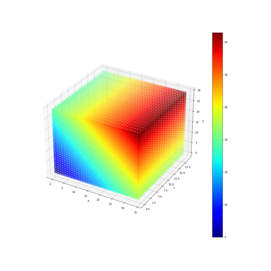
I'm not quite shure what the graphics in your code shows us. So check it out carefully by using different initialisations for T (or w2) and with kx, ky, kz values that are not all the same. Note the indexing="ij" option in the np.meshgrid() command. The use of np.nan is somehow dangerous because it changes the variable globaly.

import numpy as np
from matplotlib import pyplot as plt
from matplotlib import cm
from mpl_toolkits.mplot3d import Axes3D

def get_grid(mx, my, mz, Lx,Ly,Lz):
    ix, iy, iz = Lx*np.linspace(0,1,mx), Ly*np.linspace(0,1,my), Lz*np.linspace(0,1,mz)
    x, y, z = np.meshgrid(ix,iy,iz, indexing='ij')
    print('ix', ix), print('iy', iy), print('iz', iz)
    return x,y,z

def plot_grid(x,y,z,T):
    def plot_boundary_only(x,y,z,T):
        mx, my, mz = x.shape
        x[1:-1, 1:-1, 1:-1],y[1:-1, 1:-1, 1:-1],z[1:-1, 1:-1, 1:-1],T[1:-1, 1:-1, 1:-1] = np.nan, np.nan, np.nan, np.nan     # remove interior
        x[1:-1, 1:,0], y[1:-1, 1:,0], z[1:-1, 1:,0],  T[1:-1, 1:,0] = np.nan, np.nan, np.nan, np.nan                         # remove bottom
        x[1:-1, my-1, 1:-1], y[1:-1, my-1, 1:-1], z[1:-1, my-1, 1:-1], T[1:-1, my-1, 1:-1] = np.nan, np.nan, np.nan, np.nan  # remove north face
        x[0, 1:, :-1], y[0, 1:, :-1], z[0, 1:, :-1], T[0, 1:, :-1] = np.nan, np.nan, np.nan, np.nan                          # remove west face
        return x,y,z,T
    
    x,y,z,T = plot_boundary_only(x,y,z,T)   
    fig = plt.figure(figsize=(15,15))
    ax = fig.add_subplot(111, projection='3d')
    img = ax.scatter(x,y,z, c=T.reshape(-1), s=150, cmap=plt.jet())
    fig.colorbar(img)
    
    #ax.zaxis.set_rotate_label(False) # To disable automatic label rotation
    ax.set_ylabel('Y')
    ax.set_xlabel('X', rotation=0)
    ax.set_zlabel('Z', rotation=0)
    plt.savefig("cube.png")
    plt.show()
    
def init_T(x,y,z):
    T = np.zeros_like(x)
    case = 'xz'
    if case == 'x': T = x
    if case == 'y': T = y
    if case == 'z': T = z
    if case == 'xz': T = x+z
    return T

nx, ny, nz = 35, 20, 30
Lx, Ly, Lz = nx-1, ny-1, nz-1
x,y,z = get_grid(nx, ny, nz, Lx,Ly,Lz)  # generate a grid with mesh size Δx = Δy = Δz = 1
T = init_T(x,y,z)
plot_grid(x,y,z,T)

This is the main program to run the the heat equation solver. Note that we can not use the grafics displaying the points at the surface to see any results! The Neumann conditions are at the bottom which we can not see, and the values at the faces are fixed value boundary conditions which do not change.

def set_GradBC(u):
    #--- Neuman BC at bottom boundary ---
    u[:, :, 0] = u[:, :, 1]
    return u


def dT(u,DU):
    DU[jxp,jyp,jzp] = (u[jxe,jyp,jzp] - 2.0*u[jxp,jyp,jzp] + u[jxw,jyp,jzp])*Dx + \
                      (u[jxp,jyn,jzp] - 2.0*u[jxp,jyp,jzp] + u[jxp,jys,jzp])*Dy + \
                      (u[jxp,jyp,jzt] - 2.0*u[jxp,jyp,jzp] + u[jxp,jyp,jzb])*Dz
    return DU

#mmmmmmmmmmmmm main mmmmmmmmmmmmmmmmmmmmmmmmmmmmmmmmmmmmmmmmmmmmmmmmm
#---- set the parameters ------------------------
dt = 0.01                                    # time step size
nIterations = 5000                           # number of iterations
nx, ny, nz = 40,20,30                       # number of grid points
Lx, Ly, Lz = nx-1, ny-1, nz-1                 # physical grid size
Kx, Ky, Kz = 1, 1, 1                          # diffusion coeficients
dx, dy, dz = Lx/(nx-1), Ly/(ny-1), Lz/(nz-1)  # mesh size
Dx, Dy, Dz = Kx/dx**2, Ky/dy**2, Kz/dz**2     # equation coefficients

#---- initialize the field variables -----------------
x,y,z = get_grid(nx, ny, nz, Lx,Ly,Lz)       # generate the grid
T = init_T(x,y,z)                            # initialize the temperature
DT = np.zeros_like(T)                        # initialize the change of temperature
jxw, jxp, jxe, \
jys, jyp, jyn, \
jzb, jzp, jzt = get_slices(nx, ny, nz)       # slices for finite differencing

#---- run the solving algorithm ----------------------
for jter in range(nIterations):
    T = set_GradBC(T)              # set Neumann boundary condition
    T = T + dt*dT(T,DT)            # update

Here is a slice displaying the result along JY1=constant:

def plot_y_slice(JY1, x,y,z,T):
    T2 = T[:,JY1,:]
    X =  x[:,JY1,:]
    Z =  z[:,JY1,:]

    fig = plt.figure(figsize=(15,15))
    ax = fig.add_subplot(111)
    ax.set_aspect('equal')
    plt.contourf(X,Z,T2, 40,alpha=0.99)
    plt.savefig("y_slice.png")
    plt.show()
    
JY1 = 10
plot_y_slice(JY1, x,y,z,T)

Biebel

When I try the main program to run the the heat equation solver. It returns the same plot as the cube from your first two codes. Is there a reference for full explanation? – Siracusa

@ Freya the Goddess: I am not sure wether I understand your question correctly. The main program does nor call any graphics. After running the main program you can call either plot_grid(x,y,z,T) which will display the cube or JY1 = 10; plot_y_slice(JY1,x,y,z,T) which will display the 2-dimensional cross section. – Biebel

When looking at the the cube you just see the boundary values of the surfaces. These boundary values are fixed on all surfaces except at the bottom iz=0. When looking at the cube in this manor you cannot see that something has changed due to the heat equation solver. Therfore you will need slices with 2-dimensional displays. – Biebel

Yes that's what I actually mean, by calling the 2-dimensional cross section is to type this at the end plot_y_slice(JY1, x,y,z,T), some codes from making 3-d cubes made me unable to plot the y-slice, I fixed it now. Thanks – Siracusa

in order to be more flexible I would like to use PyVista for that , having more flxibility in 3 dimensions than Matplaplotli which is excellent for 2 dimensions – Biebel

Answer 3

There's an error in your equation for the Neumann BC, the diffusion constant is missing. This lines

#Neumann boundary (dx=dy=dz for the time)
        w2[0,:,:] =   w2[0,:,:] + 2*kapp* (dt4/(dx4**2)) * (w2[1,:,:] - w2[0,:,:] - qq1 * dx4/kapp)
        w2[-1,:,:] =  w2[-1,:,:] + 2* kapp*(dt4/(dx4**2)) * (w2[-2,:,:] - w2[-1,:,:] + qq2 * dx4/kapp)
        w2[:,0,:] =   w2[:,0,:] + 2*kapp* (dt4/(dx4**2)) * (w2[:,1,:] - w2[:,0,:] - qq3 * dx4/kapp)
        w2[:,-1,:] =  w2[:,-1,:] + 2*kapp* (dt4/(dx4**2)) * (w2[:,-2,:] - w2[:,-1,:] + qq4 * dx4/kapp)
        w2[:,:,0] =   w2[:,:,0] + 2 *kapp* (dt4/(dx4**2)) * (w2[:,:,-1] - w2[:,:,0] - qq5 * dx4/kapp)
        w2[:,:,-1] =   w2[:,:,-1] + 2 *kapp* (dt4/(dx4**2)) * (w2[:,:,-2] - w2[:,:,-1] + qq6 * dx4/kapp)

Should be changed to

#Neumann boundary (dx=dy=dz for the time)
        w2[0,:,:] =   w2[0,:,:] + 2*kapp* (dt4/(dx4**2)) * (w2[1,:,:] - w2[0,:,:] - qq1 * dx4)
        w2[-1,:,:] =  w2[-1,:,:] + 2* kapp*(dt4/(dx4**2)) * (w2[-2,:,:] - w2[-1,:,:] + qq2 * dx4)
        w2[:,0,:] =   w2[:,0,:] + 2*kapp* (dt4/(dx4**2)) * (w2[:,1,:] - w2[:,0,:] - qq3 * dx4)
        w2[:,-1,:] =  w2[:,-1,:] + 2*kapp* (dt4/(dx4**2)) * (w2[:,-2,:] - w2[:,-1,:] + qq4 * dx4)
        w2[:,:,0] =   w2[:,:,0] + 2 *kapp* (dt4/(dx4**2)) * (w2[:,:,-1] - w2[:,:,0] - qq5 * dx4)
        w2[:,:,-1] =   w2[:,:,-1] + 2 *kapp* (dt4/(dx4**2)) * (w2[:,:,-2] - w2[:,:,-1] + qq6 * dx4)

Friedrich