How to use a named column in Excel formulas

Question

I know how to make a named range in Excel.

I have a spreadsheet, with various columns going across as parameters, and then finally a formula in the last cell. This is repeated many times in each row, with each row having a different set of data, and the formula updated to reference the correct row index.

However, the formula looks like (three rows worth):

=G2*(10*D2 + 20*E2 + 5*F2)
=G3*(10*D3 + 20*E3 + 5*F3)
=G4*(10*D4 + 20*E4 + 5*F4)

I would like to use named ranges, but I can't find a way to do something like

=Count * (10*var1 + 20*var2 + 5*var3)

where count, var1, var2, and var3 automatically update to be the particular column of the current row. I can create a named range for every cell, but that isn't helpful. I can name range the column, but then I can't find a way to put an offset into the formula.

Also the whole point of this is readability, so if it ends up being some nasty complex formula function call, that probably doesn't help too much.

Gramps

Answer 1

Suppose I have the following numbers set up in columns D to F in rows 2 to 4:

    D    E    F    G
2   10   15   20
3   1    2    3
4   20   30   40

Now suppose I want the value in column D to be known as input1, column E to be input2, and column F to input3:

In Insert > Name > Define...

input1 RefersTo =OFFSET(Sheet1!$D$2,0,0,COUNT(Sheet1!$D:$D),1)
input2 RefersTo =OFFSET(Sheet1!$E$2,0,0,COUNT(Sheet1!$E:$E),1)
input3 RefersTo =OFFSET(Sheet1!$F$2,0,0,COUNT(Sheet1!$F:$F),1)

Now if I write my formula in column G as follows I should get correct answers:

G2 =(10*input1+20*input2+30*input3) // 1000
G3 =(10*input1+20*input2+30*input3) // 140
G5 =(10*input1+20*input2+30*input3) // 2000

Uropygium

One would think after 30 years of development, Microsoft would have thought of a more intuitive way to solve this problem. – Hereld

After 30+4 I cannot find how to apply this workaround... How can I do it using Excel 2010? – Indole

Answer 2

Simple, at least when using Excel 2010:

1. name your column: select full column, enter name
2. use column name in formula; Excel will combine the referenced column with the current row to access a single cell.

Using the example from Alex P:

1. select column D by clicking the column header containing the "D", enter name "input1" into name field, and press Enter.
2. repeat for columns E to F, using "input2" and "input3", respectively.
3. Do not define additional names defining names "input1" [...] as in example above!
4. use the formula as given in the example above

Attention:

Using named columns this way, you cannot access any other row as the one your formula is in!

At least I'm not aware of the possibility to express something like <ColName>(row+1)...

Xe

Answer 3

I would suggest creating a Table. Select your range A1:H4, then go to the Tables widget > New > Insert Table with Headers (on Mac). This will mark A2:H4 as body of the table, and A1:H4 as header.

From that, you get:

• Whatever you put into the header column will define the name for this column automatically, e.g. Count, Radius, Density, Height
• You can then write your formula using =[@Count]*(10*[@Radius] + 20*[@Density] + 5*[@Height])
• When you change the formula in cell H2, Excel will automatically "copy down" this formula to all cells in column H. So no more accidental inconsistencies in the formulas.
• When you need to add another row, simply click the last cell (in our example H4) and hit Tab. Excel adds another row, and also makes sure to "copy down" your formula into the new row.
• If you need a total row, add it with the Total Row checkbox in the Tables widget. Excel adds a total row automatically. If you click any cell in the total row, you can change the "total formula" with the "▼▲" button, for example to calculate the Average instead of the Sum of the column.
• If you have a long table and scroll down so that the header is not visible anymore, Excel automatically displays the column header instead of the column names (Count instead of G for example).

I can really recommend the video You Suck at Excel with Joel Spolsky which explains all of that.

Illiterate

Answer 4

I haven't fully reviewed the previous answers, but I think this is closer to what @Jason Coyne the OP was looking for. So, I hope I get a lot of up votes. ;-)

Excel allows your formula to refer to tables and columns by name if you "Format as Table". Here is an article titled Using structured references with Excel tables that goes into detail.

FWIW, it looks like this feature has been available since Excel 2007.

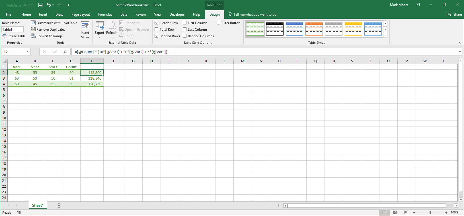
Here is a screenshot of an example:

You should be able to see the formula in E2 is =[@Count] * (10*[@Var1] + 20*[@Var2] + 5*[@Var3]) which is pretty close to what @jason-coyne wanted to type.

I don't like that you are forced to pick a style (or define a new one if you don't see a style you like). The good news is you can reformat the cells all you wish without undoing the "tableness".

It insists on turning on auto-filter. But, auto filter is easy to turn off (see the Filter Button checkbox under the Table Tools Design menu).

It also insists on having non-empty, unique values in the header row (Which kinda makes sense). If you delete a header cell, or insert a column, Excel will invent a new, unique name and stuff it in for you. D'oh!

If you want a column to not have a header, you can enter an apostrophe (') followed by one or more blanks. Remember header values need to be unique, so keep adding blanks if you want more than one column without a header.

If you would like to download the sample workbook in the screenshot, here is a link: https://filebin.ca/3vfaSDn4NLEA/SampleWorkbook.xlsx

Reachmedown

Avoid including external links, just include the dataset directly here. – Susuable

@adriano-martins, I don't see how to add a dataset directly to an answer. Would you mind adding a comment or a link to explain how to do that? FWIW, I really needed to include an XLSX file because the key to implementing what the OP was asking for is formatting the table. As I'm not sure what a directly attached "dataset" means (yet), I'm guessing it does not include the formatting of the cells. Looking forward to learning how to add a dataset directly to an answer. – Reachmedown

The column name takes properly for the current row, but if I want to refer to one row above then it refer to D1,D2 instead of column name. Any idea how to do it ? – Pelvis

Answer 5

Adding to Alex P's answer:

Instead of using

=OFFSET(Sheet1!$D$2,0,0,COUNT(Sheet1!$D:$D),1)

as the formula for input1, I recommend to use

=Sheet1!$D$2:INDEX(Sheet1!$D:$D,COUNT(Sheet1"$D:$D))

It produces the same result, but it is non-volatile, i.e., only recalculate when a predecessor cell changes. This is much better in a larger model!

Enchorial

Answer 6

If you're using VBA, then you can select the whole column and name it, say MyCol, in the name box (upper left input box). The in your code you can refer to a cell in the column MyCol (line 12) using the following code:

Cells(12, Range("MyCol").Column)

Indole

Answer 7

You might be able to use the row() function. This returns the current row that you are in. So depending on the layout of the spreadsheet you can use it like this:

=offset(NamedColumn1, row()-1)

The -1 is because you are saying how many rows to move down from row 1 which if you are in row 1 you want to be 0.

Cathar

Answer 8

Use the Excel feature called named references.

To name a cell or range of cells

1. select that cell or range of cells
2. Enter its name in the Name Box ( its left of the formula widget and has the cell name )

You can't use names that conflict with cell names, like k0.

The named cells can be used if formulas. E.g.,

=pi*radius*radius

Subtotal

The link is broken ("Sorry, the page you’re looking for can’t be found."). – Apodaca

Answer 9

I'd like to propose a slight variation of the cell reference made by Dror. This will work as well:

Range("MyCol").Rows(12)

Durant