Implementing log Gabor filter bank

Question

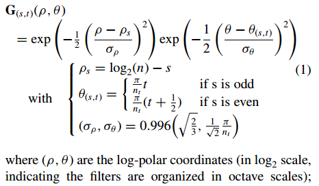
I was reading this paper "Self-Invertible 2D Log-Gabor Wavelets" it defines 2D log gabor filter as such:

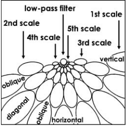
The paper also states that the filter only covers one side of the frequency space and shows that in this image

On my attempt to implement the filter I get results that do not match with what is said in the paper. Let me start with my implementation then I will state the problems.

Implementation:

1. I created a 2d array that contains the filter and transformed each index so that the origin of the frequency domain is at the center of the array with positive x-axis going right and positive y-axis going up.

   number_scales = 5         # scale resolution
   number_orientations = 9   # orientation resolution
   N = constantDim           # image dimensions
   
   def getLogGaborKernal(scale, angle, logfun=math.log2, norm = True):
       # setup up filter configuration
       center_scale = logfun(N) - scale          
       center_angle = ((np.pi/number_orientations) * angle) if (scale % 2) \
                   else ((np.pi/number_orientations) * (angle+0.5))
       scale_bandwidth =  0.996 * math.sqrt(2/3)
       angle_bandwidth =  0.996 * (1/math.sqrt(2)) * (np.pi/number_orientations)
   
       # 2d array that will hold the filter
       kernel = np.zeros((N, N))
       # get the center of the 2d array so we can shift origin
       middle = math.ceil((N/2)+0.1)-1
   
       # calculate the filter
       for x in range(0,constantDim):
           for y in range(0,constantDim):
               # get the transformed x and y where origin is at center
               # and positive x-axis goes right while positive y-axis goes up
               x_t, y_t = (x-middle),-(y-middle)
               # calculate the filter value at given index
               kernel[y,x] = logGaborValue(x_t,y_t,center_scale,center_angle,
           scale_bandwidth, angle_bandwidth,logfun)
   
       # normalize the filter energy
       if norm:
           Kernel = kernel / np.sum(kernel**2)
       return kernel
   

2. To calculate the filter value at each index another transform is made where we go to the log-polar space

   def logGaborValue(x,y,center_scale,center_angle,scale_bandwidth,
                 angle_bandwidth, logfun):
       # transform to polar coordinates
       raw, theta = getPolar(x,y)
       # if we are at the center, return 0 as in the log space
       # zero is not defined
       if raw == 0:
           return 0
   
       # go to log polar coordinates
       raw = logfun(raw)
   
       # calculate (theta-center_theta), we calculate cos(theta-center_theta) 
       # and sin(theta-center_theta) then use atan to get the required value,
       # this way we can eliminate the angular distance wrap around problem
       costheta, sintheta = math.cos(theta), math.sin(theta)
       ds = sintheta * math.cos(center_angle) - costheta * math.sin(center_angle)    
       dc = costheta * math.cos(center_angle) + sintheta * math.sin(center_angle)  
       dtheta = math.atan2(ds,dc)
   
       # final value, multiply the radial component by the angular one
       return math.exp(-0.5 * ((raw-center_scale) / scale_bandwidth)**2) * \
               math.exp(-0.5 * (dtheta/angle_bandwidth)**2)
   

Problems:

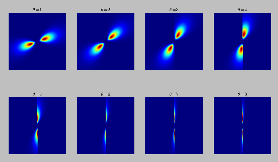
1. The angle: the paper stated that indexing the angles from 1->8 would produce good coverage of the orientation, but in my implementation angles from 1->n don't cover except for half orientations. Even the vertical orientation is not correctly covered. This can be shown in this figure which contains sets of filters of scale 3 and orientations ranging from 1->8:

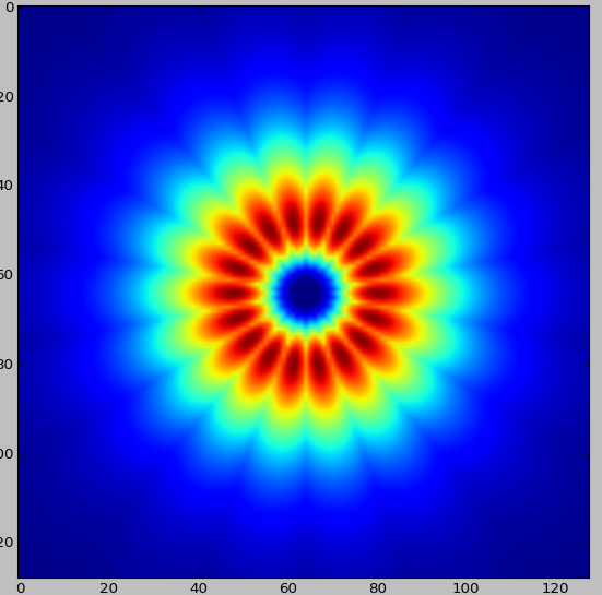
2. The coverage: from filters above it is clear the filter covers both sides of the space which is not what the paper says. This can be made more explicit by using 9 orientations ranging from -4 -> 4. The following image contains all the filters in one image to show how it covers both sides of the spectrum (this image is created by taking the maximum at each location from all filters):

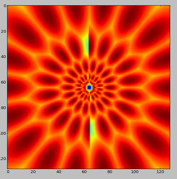
3. Middle Column (orientation $\pi / 2$): in the first figure in orientation from 3 -> 8 it can be seen that the filter vanishes at orientation $ \pi / 2$. Is this normal? This can be seen too when I combine all the filters(of all 5 scales and 9 orientations) in one image:

Update: Adding the impulse response of the filter in spatial domain, as you can see there is an obvious distortion in -4 & 4 orientations:

Topdrawer

Answer 1

After a lot of code analysis, I found that my implementation was correct but the getPolar function was messed up, so the code above should work just fine. This is the a new code without the getPolar function if any one was looking for it:

number_scales = 5          # scale resolution
number_orientations = 8    # orientation resolution
N = 128                    # image dimensions
def getFilter(f_0, theta_0):
    # filter configuration
    scale_bandwidth =  0.996 * math.sqrt(2/3)
    angle_bandwidth =  0.996 * (1/math.sqrt(2)) * (np.pi/number_orientations)

    # x,y grid
    extent = np.arange(-N/2, N/2 + N%2)
    x, y = np.meshgrid(extent,extent)

    mid = int(N/2)
    ## orientation component ##
    theta = np.arctan2(y,x)
    center_angle = ((np.pi/number_orientations) * theta_0) if (f_0 % 2) \
                else ((np.pi/number_orientations) * (theta_0+0.5))

    # calculate (theta-center_theta), we calculate cos(theta-center_theta) 
    # and sin(theta-center_theta) then use atan to get the required value,
    # this way we can eliminate the angular distance wrap around problem
    costheta = np.cos(theta)
    sintheta = np.sin(theta)
    ds = sintheta * math.cos(center_angle) - costheta * math.sin(center_angle)    
    dc = costheta * math.cos(center_angle) + sintheta * math.sin(center_angle)  
    dtheta = np.arctan2(ds,dc)

    orientation_component =  np.exp(-0.5 * (dtheta/angle_bandwidth)**2)

    ## frequency componenet ##
    # go to polar space
    raw = np.sqrt(x**2+y**2)
    # set origin to 1 as in the log space zero is not defined
    raw[mid,mid] = 1
    # go to log space
    raw = np.log2(raw)

    center_scale = math.log2(N) - f_0
    draw = raw-center_scale
    frequency_component = np.exp(-0.5 * (draw/ scale_bandwidth)**2)

    # reset origin to zero (not needed as it is already 0?)
    frequency_component[mid,mid] = 0

    return frequency_component * orientation_component

Topdrawer

Thank you for replying to your own question. I was also looking for an information concerning log gabor filters for iris recognition and found your post very useful – Inveigh

Answer 2

Yes - this was very helpful for me as well. As I was just learning about log-gabor filters, it took me a bit to realize a few things that maybe are basic, but I figured I'd mention it here for others. Log-gabor is a frequency filter. So rather than making a small kernel and convolving across the image, you just multiply it in frequency space.

That means that N must match the image size, and that you must first transform with fft, then just multiply the filter, then transform back with inverse fft. This code gave me what I needed to get a full end-to-end test, filtering an image. I could then render the resulting images and verify I was getting what I expected. As a test, 3 orientations can be easily visualized by merging into a single RGB image.

def fft(im):
    return np.fft.fftshift(np.fft.fft2(im))

def ifft(f):
    return np.real(np.fft.ifft2(np.fft.ifftshift(f)))

N = src.shape[0]
f_0 = 4
number_orientations = 4
lg = [getLogGaborFilter(N,f_0,x,number_orientations) for x in range(0,number_orientations)]
f = [ifft(fft(src) * lg[x]) for x in range(0,number_orientations)]

I changed the function signature a bit, to take image size and number of orientations. Also, it took me a bit to realize what f_0 was exactly. From math.log2(N) - f_0, this is the equivalent of dividing N by 2 to the power of f_0, selecting for larger and larger scale features. My understanding is this means you probably just want to use small positive integers.

Midrash