Fit Curve-Spline to 3D Point Cloud

Question

Objective

I have a 3D facet model (e.g. .off file) which can for example look like a pipe/tube (see example picture). The goal is to derive an approximate spline (best case combination of lines and splines) which represents the 3D skeleton of this tube using python.

State of the art

Stackoverflow posts in same field:

• how-to-fit-a-line-through-a-3d-pointcloud

General:

• Fitting-Spline-Curves-through-Set-of-Unorganized Point Cloud
• Skeletons from point cloud
• Powercrust / NN-Crust? I read about those, however I cant find a python implementation and maybe I am too dumb to implement it on my own. As far as I understood, the basis is delaunay/voronoi which I know already. However i dont know any further steps

My Approach (so far)

Starting from the example facet model (Image 1), I used a python package to convert the 3d model to a point cloud (Image 2). This point cloud can be used for a voxelized representation (Image 3). Consequently, these three types of data are my starting point.

Basically, this problem does not seem too complicated to me, however I am missing a starting logic. Most of the research papers overcomplicate this for various further-reaching tasks. One idea would be to do a PCA to derive major axes of the component, and scan along these axes. However, this doesnt appear to lead to good results in a performant way. Another idea would be to use the voxelized grid and detect a path due to voxel adjacencies. Another idea would be to use KD-Tree to evaluate closest points to detect the correct planes for defining the spline direction via their plane normals.

An approach that I tried was to select N random points from the pointcloud and search for all neighbors within a radius (cKDTree.query_ball_point). I calculated the center of all neighboring points. This leads to the result in image 4. The result seems good as first approach, however it is more or less a tuning of the radius parameter.

Image 1:

Image 2:

Image 3:

Image 4:

Cassatt

Are the facets in your surface model structured (e.g., all quads - or triangulated quads - with one edge along the tube direction)? – Sundae

I dont think so, or at least I dont want to take that as granted as it depicts another boundary condition. I will add another try of me in the question now – Cassatt

Answer 1

Delaunay/Voronoi methods can be used for this problem, since the medial axis is a sub-graph of the Voronoi graph (see for example this paper by Attali, Boissonnat and Edelsbrunner).

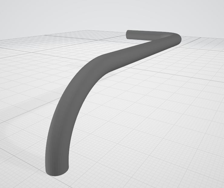
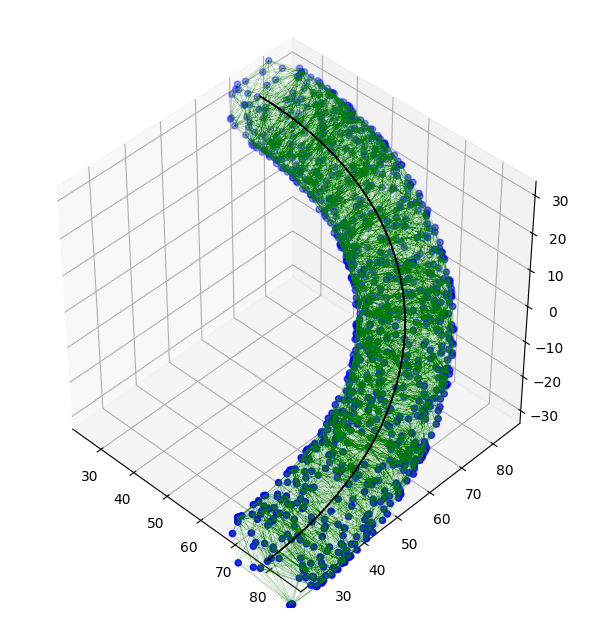
In the following I will demonstrate the methods on an example of points sampled from a quarter torus surface with small radius 10 and large radius 100 (the medial path/skeleton starts at point (100, 0, 0) and ends at (0, 100, 0)).

The Voronoi graph is the dual of the 3D Delaunay tetrahedralization (I will from now on use the term triangulation for this). Computing the Delaunay triangulation can be done using scipy's scipy.spatial.Delaunay package.

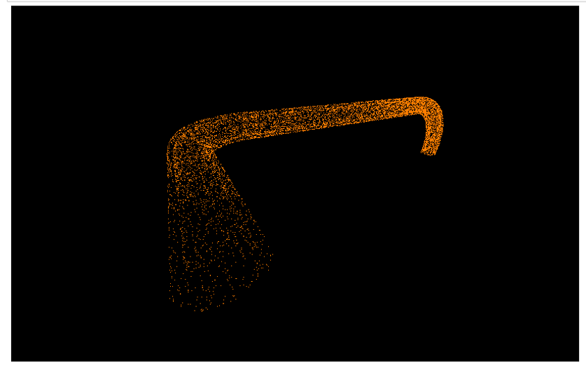
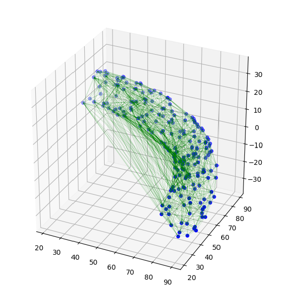
Below is a figure of the sample points (200 in this example) and their full Delaunay triangulation (the triangulation was plotted with the function from here).

The Voronoi vertex corresponding to a Delaunay tetrahedron is the center of the circumscribing sphere of the tetrahedron. The following is a function that computes these Delaunay centers, it is an extension to the 2D function from my previous answer here.

def compute_delaunay_tetra_circumcenters(dt):
"""
Compute the centers of the circumscribing circle of each tetrahedron in the Delaunay triangulation.
:param dt: the Delaunay triangulation
:return: array of xyz points
"""
simp_pts = dt.points[dt.simplices]
# (n, 4, 3) array of tetrahedra points where simp_pts[i, j, :] holds the j'th 3D point (of four) of the i'th tetrahedron
assert simp_pts.shape[1] == 4 and simp_pts.shape[2] == 3

# finding the circumcenter (x, y, z) of a simplex defined by four points:
# (x-x0)**2 + (y-y0)**2 + (z-z0)**2 = (x-x1)**2 + (y-y1)**2 + (z-z1)**2
# (x-x0)**2 + (y-y0)**2 + (z-z0)**2 = (x-x2)**2 + (y-y2)**2 + (z-z2)**2
# (x-x0)**2 + (y-y0)**2 + (z-z0)**2 = (x-x3)**2 + (y-y3)**2 + (z-z3)**2
# becomes three linear equations (squares are canceled):
# 2(x1-x0)*x + 2(y1-y0)*y + 2(z1-z0)*y = (x1**2 + y1**2 + z1**2) - (x0**2 + y0**2 + z0**2)
# 2(x2-x0)*x + 2(y2-y0)*y + 2(z2-z0)*y = (x2**2 + y2**2 + z2**2) - (x0**2 + y0**2 + z0**2)
# 2(x3-x0)*x + 2(y3-y0)*y + 2(z3-z0)*y = (x3**2 + y3**2 + z3**2) - (x0**2 + y0**2 + z0**2)

# building the 3x3 matrix of the linear equations
a = 2 * (simp_pts[:, 1, 0] - simp_pts[:, 0, 0])
b = 2 * (simp_pts[:, 1, 1] - simp_pts[:, 0, 1])
c = 2 * (simp_pts[:, 1, 2] - simp_pts[:, 0, 2])
d = 2 * (simp_pts[:, 2, 0] - simp_pts[:, 0, 0])
e = 2 * (simp_pts[:, 2, 1] - simp_pts[:, 0, 1])
f = 2 * (simp_pts[:, 2, 2] - simp_pts[:, 0, 2])
g = 2 * (simp_pts[:, 3, 0] - simp_pts[:, 0, 0])
h = 2 * (simp_pts[:, 3, 1] - simp_pts[:, 0, 1])
i = 2 * (simp_pts[:, 3, 2] - simp_pts[:, 0, 2])

v1 = (simp_pts[:, 1, 0] ** 2 + simp_pts[:, 1, 1] ** 2 + simp_pts[:, 1, 2] ** 2) - (simp_pts[:, 0, 0] ** 2 + simp_pts[:, 0, 1] ** 2 + simp_pts[:, 0, 2] ** 2)
v2 = (simp_pts[:, 2, 0] ** 2 + simp_pts[:, 2, 1] ** 2 + simp_pts[:, 2, 2] ** 2) - (simp_pts[:, 0, 0] ** 2 + simp_pts[:, 0, 1] ** 2 + simp_pts[:, 0, 2] ** 2)
v3 = (simp_pts[:, 3, 0] ** 2 + simp_pts[:, 3, 1] ** 2 + simp_pts[:, 3, 2] ** 2) - (simp_pts[:, 0, 0] ** 2 + simp_pts[:, 0, 1] ** 2 + simp_pts[:, 0, 2] ** 2)

# solve a 3x3 system by inversion (see https://en.wikipedia.org/wiki/Invertible_matrix#Inversion_of_3_%C3%97_3_matrices)
A = e*i - f*h
B = -(d*i - f*g)
C = d*h - e*g
D = -(b*i - c*h)
E = a*i - c*g
F = -(a*h - b*g)
G = b*f - c*e
H = -(a*f - c*d)
I = a*e - b*d

det = a*A + b*B + c*C

# multiplying inv*[v1, v2, v3] to get solution point (x, y, z)
x = (A*v1 + D*v2 + G*v3) / det
y = (B*v1 + E*v2 + H*v3) / det
z = (C*v1 + F*v2 + I*v3) / det

return (np.vstack((x, y, z))).T

We would like to filter out tetrahedra that are outside of the original surface (see for example the long tetrahedra in the figure above). This might be done by testing the tetrahedra against the original surface. However, a simpler way, which is very suited for the input of a tube/pipe surface is to filter out tetrahedra that have a large circumscribing radius. This is what the alpha-shape algorithm does. This is easily done within our context since the radius is just the distance between the center and any of the tetrahedron points.

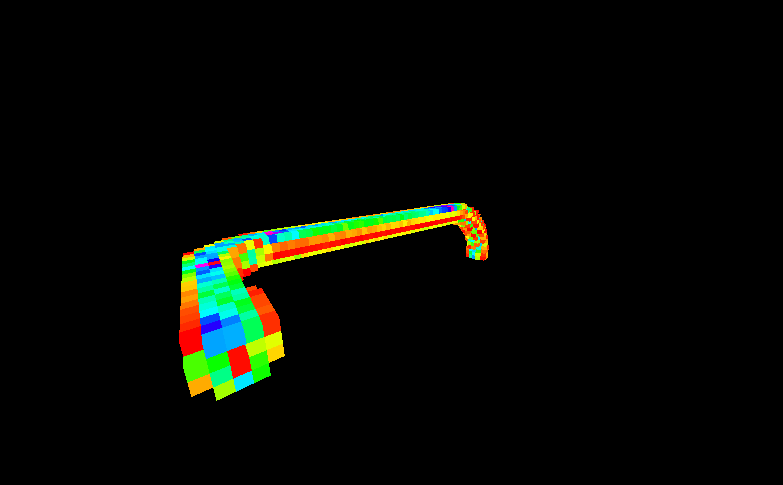
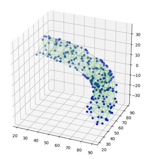
The following figure shows the Delaunay triangulation after filtering out tetrahedra with radius greater than 20.

We can now use these building blocks to build the Voronoi sub-graph of the tetrahedra that pass the radius condition. The function below does this using the connectivity information in the Delaunay triangulation to construct the Voronoi sub-graph, represented as an edge list.

def compute_voronoi_vertices_and_edges(points, r_thresh=np.inf):
"""
Compute (finite) Voronoi edges and vertices of a set of points.
:param points: input points.
:param r_thresh: radius value for filtering out vertices corresponding to
Delaunay tetrahedrons with large radii of circumscribing sphere (alpha-shape condition).
:return: array of xyz Voronoi vertex points and an edge list.
"""
dt = Delaunay(points)
xyz_centers = compute_delaunay_tetra_circumcenters(dt)

# filtering tetrahedrons that have radius > thresh
simp_pts_0 = dt.points[dt.simplices[:, 0]]
radii = np.linalg.norm(xyz_centers - simp_pts_0, axis=1)
is_in = radii < r_thresh

# build an edge list from (filtered) tetrahedrons neighbor relations
edge_lst = []
for i in range(len(dt.neighbors)):
    if not is_in[i]:
        continue  # i is an outside tetra
    for j in dt.neighbors[i]:
        if j != -1 and is_in[j]:
            edge_lst.append((i, j))

return xyz_centers, edge_lst

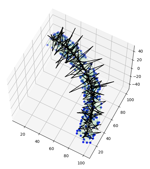
The result is still not sufficient as can be seen in the figure below, where the sub-graph edges are the black line segments. The reason is that 3D Delaunay triangulations are notorious for having thin tetrahedra (so-called slivers, needles and caps in this paper by Shewchuk), which cause the outer "spikes" in the results.

While there are general methods to remove these unwanted spikes (see, for example, Amenta and Bern), in the context of a tube surface there is a simple solution. The path we are looking for can be computed as the shortest Euclidean path in the graph starting at the closest point to the start of the tube and ending at the closest point to the end. The following code does this using a networkx graph with weights set to the lengths of the edges.

# get closest vertex to start and end points
xyz_centers, edge_lst = compute_voronoi_vertices_and_edges(pts, r_thresh=20.)
kdt = cKDTree(xyz_centers)
dist0, idx0 = kdt.query(np.array([100., 0, 0]))
dist1, idx1 = kdt.query(np.array([0, 100., 0]))

# compute shortest weighted path
edge_lengths = [np.linalg.norm(xyz_centers[e[0], :] - xyz_centers[e[1], :]) for e in edge_lst]
g = nx.Graph((i, j, {'weight': dist}) for (i, j), dist in zip(edge_lst, edge_lengths))
path_s = nx.shortest_path(g,source=idx0,target=idx1, weight='weight')

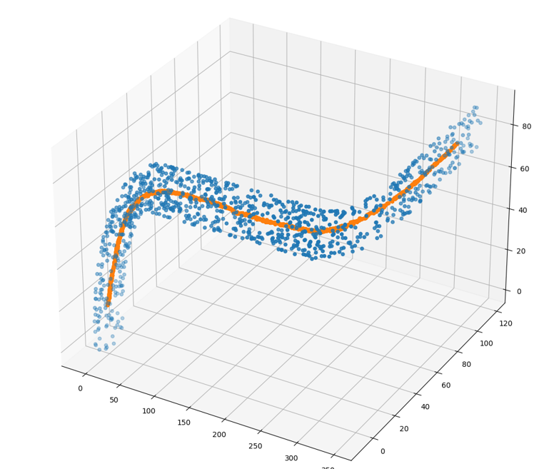
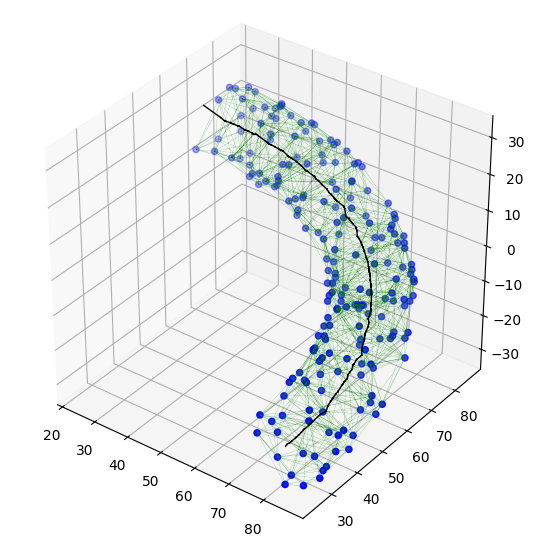
The figure below shows the results for the original 200 points.

And this is the results for a denser sample of 1000 points.

Now you can pass an approximating spline - interpolating or least-square fit, through the path points. You can use scipy.interpolate.UnivariateSpline as suggested in the link or scipy.interpolate.splrep as done here or any other standard spline implementation.

Heurlin

Thank you @Iddo Hanniel for your great effort! This seems really promising. The only downturn is that one has to tune the distance parameter, but it really seems like a good solution. Unfortunately, I dont have much spare time right now, will test it as soon as possible! – Cassatt

Hello! I am not sure what to do with the path_s object. nx.shortest_path returns a list of integers which go higher than the length of my original input data. What do those integers mean and how do I get the coordinates of the black line shown in the last two plots? Thank you! – Showalter

The path_s object is a list of indices in the xyz_centers array. So [xyz_centers[i, :] for i in path_s] should give you the list of (ordered) 3d coordinates of the black line. – Heurlin

@Cassatt old thread, but tagging on to this answer. You can use the medial axis transform of your mesh, then use a mean curvature flow (MCF) filter to bring it down to a skeleton. There are several "skeletonize" repos on github that do just this. I found some after trying to re-invent the wheel myself! – Cassilda

I'm not sure what your data is, but the first and last points of the path in the example code above (points closest to [100., 0, 0] and [0, 100, 0]) are tailored to this specific torus example. Therefore I'd be surprised if they are suitable for your data. In your code you should use source and target points that are suitable for your own problem. See also my comment to the following answer, which discusses this. https://mcmap.net/q/1164023/-how-can-i-fit-a-curve-to-a-3d-point-cloud – Heurlin

@IddoHanniel Thanks, that was a very obvious mistake from my end, the answer is very clearly written! In your comment over the mentioned post you have mentioned using PCA for a shape resembling a cylinder, what if there's a distribution similar to the one mentioned in the question? Can extracting a best fitting bounding box around the point cloud and extracting one of points that lie on the box's surface be a suitable approach? – Montserrat

Or @IddoHanniel I am using tree = cKDTree(points) dist_matrix = tree.sparse_distance_matrix(tree, max_distance=np.inf) which works well but produces some error on the point cloud edge. – Montserrat

An oriented bbox might work - it must be oriented and not axis-aligned since the cylinder may not necessarily be axis-aligned (unless in your specific problem it is). The farthest points can also work (again assuming an elongated cylinder shape), but the two points probably sit on the boundary so not close to the medial-axis. The PCA approach I suggested takes the farthest points, but along the longest axis, which corresponds more-or-less to the medial axis of a cylinder. Even there I'd take some average of the points near the ends. – Heurlin

@IddoHanniel Sorry to bother you again, can we tune the algorithm to work for point distributions similar to this example where we have a branched distribution. Skeletonization algorithms will work better? – Montserrat

@Montserrat I think the basic ideas can be used up to building the geometric graph (with the spikes as shown in the third figure above). However, pruning the spikes from the graph and building the "clean graph" will require some other heuristics (the shortest path method will not work). For example removing the spikes with geometric methods (e.g., something from the Amenta references I mention) or with graph methods by removing "short paths" that end at graph leaves. Hope this helps. – Heurlin